Posts
-
Deep Reinforcement Learning Doesn't Work Yet
CommentsJune 24, 2018 note: If you want to cite an example from the post, please cite the paper which that example came from. If you want to cite the post as a whole, you can use the following BibTeX:
@misc{rlblogpost,
    title={Deep Reinforcement Learning Doesn't Work Yet},
    author={Irpan, Alex},
    howpublished={\url{https://www.alexirpan.com/2018/02/14/rl-hard.html}},
    year={2018}
}
This mostly cites papers from Berkeley, Google Brain, DeepMind, and OpenAI from the past few years, because that work is most visible to me. I’m almost certainly missing stuff from older literature and other institutions, and for that I apologize - I’m just one guy, after all.
Introduction
Once, on Facebook, I made the following claim.
Whenever someone asks me if reinforcement learning can solve their problem, I tell them it can’t. I think this is right at least 70% of the time.

Deep reinforcement learning is surrounded by mountains and mountains of hype. And for good reasons! Reinforcement learning is an incredibly general paradigm, and in principle, a robust and performant RL system should be great at everything. Merging this paradigm with the empirical power of deep learning is an obvious fit. Deep RL is one of the closest things that looks anything like AGI, and that’s the kind of dream that fuels billions of dollars of funding.
Unfortunately, it doesn’t really work yet.
Now, I believe it can work. If I didn’t believe in reinforcement learning, I wouldn’t be working on it. But there are a lot of problems in the way, many of which feel fundamentally difficult. The beautiful demos of learned agents hide all the blood, sweat, and tears that go into creating them.
Several times now, I’ve seen people get lured by recent work. They try deep reinforcement learning for the first time, and without fail, they underestimate deep RL’s difficulties. Without fail, the “toy problem” is not as easy as it looks. And without fail, the field destroys them a few times, until they learn how to set realistic research expectations.
This isn’t the fault of anyone in particular. It’s more of a systemic problem. It’s easy to write a story around a positive result. It’s hard to do the same for negative ones. The problem is that the negative ones are the ones that researchers run into the most often. In some ways, the negative cases are actually more important than the positives.
In the rest of the post, I explain why deep RL doesn’t work, cases where it does work, and ways I can see it working more reliably in the future. I’m not doing this because I want people to stop working on deep RL. I’m doing this because I believe it’s easier to make progress on problems if there’s agreement on what those problems are, and it’s easier to build agreement if people actually talk about the problems, instead of independently re-discovering the same issues over and over again.
I want to see more deep RL research. I want new people to join the field. I also want new people to know what they’re getting into.
Before getting into the rest of the post, a few remarks.
-
I cite several papers in this post. Usually, I cite the paper for its compelling negative examples, leaving out the positive ones. This doesn’t mean I don’t like the paper. I like these papers - they’re worth a read, if you have the time.
-
I use “reinforcement learning” and “deep reinforcement learning” interchangeably, because in my day-to-day, “RL” always implicitly means deep RL. I am criticizing the empirical behavior of deep reinforcement learning, not reinforcement learning in general. The papers I cite usually represent the agent with a deep neural net. Although the empirical criticisms may apply to linear RL or tabular RL, I’m not confident they generalize to smaller problems. The hype around deep RL is driven by the promise of applying RL to large, complex, high-dimensional environments where good function approximation is necessary. It is that hype in particular that needs to be addressed.
-
This post is structured to go from pessimistic to optimistic. I know it’s a bit long, but I’d appreciate it if you would take the time to read the entire post before replying.
Without further ado, here are some of the failure cases of deep RL.
Deep Reinforcement Learning Can Be Horribly Sample Inefficient
The most well-known benchmark for deep reinforcement learning is Atari. As shown in the now-famous Deep Q-Networks paper, if you combine Q-Learning with reasonably sized neural networks and some optimization tricks, you can achieve human or superhuman performance in several Atari games.
Atari games run at 60 frames per second. Off the top of your head, can you estimate how many frames a state of the art DQN needs to reach human performance?
The answer depends on the game, so let’s take a look at a recent Deepmind paper, Rainbow DQN (Hessel et al, 2017). This paper does an ablation study over several incremental advances made to the original DQN architecture, demonstrating that a combination of all advances gives the best performance. It exceeds human-level performance on over 40 of the 57 Atari games attempted. The results are displayed in this handy chart.
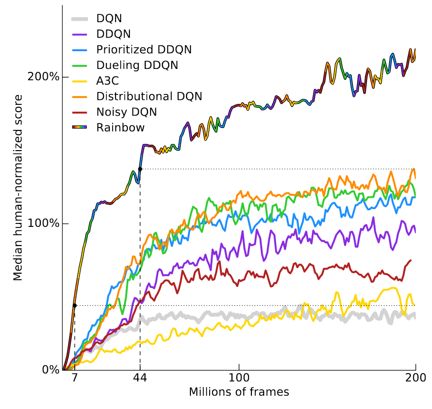
The y-axis is “median human-normalized score”. This is computed by training 57 DQNs, one for each Atari game, normalizing the score of each agent such that human performance is 100%, then plotting the median performance across the 57 games. RainbowDQN passes the 100% threshold at about 18 million frames. This corresponds to about 83 hours of play experience, plus however long it takes to train the model. A lot of time, for an Atari game that most humans pick up within a few minutes.
Mind you, 18 million frames is actually pretty good, when you consider that the previous record (Distributional DQN (Bellemare et al, 2017)) needed 70 million frames to hit 100% median performance, which is about 4x more time. As for the Nature DQN (Mnih et al, 2015), it never hits 100% median performance, even after 200 million frames of experience.
The planning fallacy says that finishing something usually takes longer than you think it will. Reinforcement learning has its own planning fallacy - learning a policy usually needs more samples than you think it will.
This is not an Atari-specific issue. The 2nd most popular benchmark is the MuJoCo benchmarks, a set of tasks set in the MuJoCo physics simulator. In these tasks, the input state is usually the position and velocity of each joint of some simulated robot. Even without having to solve vision, these benchmarks take between \(10^5\) to \(10^7\) steps to learn, depending on the task. This is an astoundingly large amount of experience to control such a simple environment.
The DeepMind parkour paper (Heess et al, 2017), demoed below, trained policies by using 64 workers for over 100 hours. The paper does not clarify what “worker” means, but I assume it means 1 CPU.
These results are super cool. When it first came out, I was surprised deep RL was even able to learn these running gaits.
At the same time, the fact that this needed 6400 CPU hours is a bit disheartening. It’s not that I expected it to need less time…it’s more that it’s disappointing that deep RL is still orders of magnitude above a practical level of sample efficiency.
There’s an obvious counterpoint here: what if we just ignore sample efficiency? There are several settings where it’s easy to generate experience. Games are a big example. But, for any setting where this isn’t true, RL faces an uphill battle, and unfortunately, most real-world settings fall under this category.
If You Just Care About Final Performance, Many Problems are Better Solved by Other Methods
When searching for solutions to any research problem, there are usually trade-offs between different objectives. You can optimize for getting a really good solution for that research problem, or you can optimize for making a good research contribution. The best problems are ones where getting a good solution requires making good research contributions, but it can be hard to find approachable problems that meet that criteria.
For purely getting good performance, deep RL’s track record isn’t that great, because it consistently gets beaten by other methods. Here is a video of the MuJoCo robots, controlled with online trajectory optimization. The correct actions are computed in near real-time, online, with no offline training. Oh, and it’s running on 2012 hardware. (Tassa et al, IROS 2012).
I think these behaviors compare well to the parkour paper. What’s different between this paper and that one?
The difference is that Tassa et al use model predictive control, which gets to perform planning against a ground-truth world model (the physics simulator). Model-free RL doesn’t do this planning, and therefore has a much harder job. On the other hand, if planning against a model helps this much, why bother with the bells and whistles of training an RL policy?
In a similar vein, you can easily outperform DQN in Atari with off-the-shelf Monte Carlo Tree Search. Here are baseline numbers from Guo et al, NIPS 2014. They compare the scores of a trained DQN to the scores of a UCT agent (where UCT is the standard version of MCTS used today.)
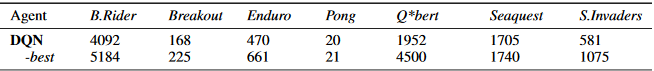
Again, this isn’t a fair comparison, because DQN does no search, and MCTS gets to perform search against a ground truth model (the Atari emulator). However, sometimes you don’t care about fair comparisons. Sometimes you just want the thing to work. (If you’re interested in a full evaluation of UCT, see the appendix of the original Arcade Learning Environment paper (Bellemare et al, JAIR 2013).)
Reinforcement learning can theoretically work for anything, including environments where a model of the world isn’t known. However, this generality comes at a price: it’s hard to exploit any problem-specific information that could help with learning, which forces you to use tons of samples to learn things that could have been hardcoded.
The rule-of-thumb is that except in rare cases, domain-specific algorithms work faster and better than reinforcement learning. This isn’t a problem if you’re doing deep RL for deep RL’s sake, but I personally find it frustrating when I compare RL’s performance to, well, anything else. One reason I liked AlphaGo so much was because it was an unambiguous win for deep RL, and that doesn’t happen very often.
This makes it harder for me to explain to laypeople why my problems are cool and hard and interesting, because they often don’t have the context or experience to appreciate why they’re hard. There’s an explanation gap between what people think deep RL can do, and what it can really do. I’m working in robotics right now. Consider the company most people think of when you mention robotics: Boston Dynamics.
This doesn’t use reinforcement learning. I’ve had a few conversations where people thought it used RL, but it doesn’t. If you look up research papers from the group, you find papers mentioning time-varying LQR, QP solvers, and convex optimization. In other words, they mostly apply classical robotics techniques. Turns out those classical techniques can work pretty well, when you apply them right.
Reinforcement Learning Usually Requires a Reward Function
Reinforcement learning assumes the existence of a reward function. Usually, this is either given, or it is hand-tuned offline and kept fixed over the course of learning. I say “usually” because there are exceptions, such as imitation learning or inverse RL, but most RL approaches treat the reward as an oracle.
Importantly, for RL to do the right thing, your reward function must capture exactly what you want. And I mean exactly. RL has an annoying tendency to overfit to your reward, leading to things you didn’t expect. This is why Atari is such a nice benchmark. Not only is it easy to get lots of samples, the goal in every game is to maximize score, so you never have to worry about defining your reward, and you know everyone else has the same reward function.
This is also why the MuJoCo tasks are popular. Because they’re run in simulation, you have perfect knowledge of all object state, which makes reward function design a lot easier.
In the Reacher task, you control a two-segment arm, that’s connected to a central point, and the goal is to move the end of the arm to a target location. Below is a video of a successfully learned policy.
Since all locations are known, reward can be defined as the distance from the end of the arm to the target, plus a small control cost. In principle, you can do this in the real world too, if you have enough sensors to get accurate enough positions for your environment. But depending on what you want your system to do, it could be hard to define a reasonable reward.
By itself, requiring a reward function wouldn’t be a big deal, except…
Reward Function Design is Difficult
Making a reward function isn’t that difficult. The difficulty comes when you try to design a reward function that encourages the behaviors you want while still being learnable.
In the HalfCheetah environment, you have a two-legged robot, restricted to a vertical plane, meaning it can only run forward or backward.
The goal is to learn a running gait. Reward is the velocity of the HalfCheetah.
This is a shaped reward, meaning it gives increasing reward in states that are closer to the end goal. This is in contrast to sparse rewards, which give reward at the goal state, and no reward anywhere else. Shaped rewards are often much easier to learn, because they provide positive feedback even when the policy hasn’t figured out a full solution to the problem.
Unfortunately, shaped rewards can bias learning. As said earlier, this can lead to behaviors that don’t match what you want. A good example is the boat racing game, from an OpenAI blog post. The intended goal is to finish the race. You can imagine that a sparse reward would give +1 reward for finishing under a given time, and 0 reward otherwise.
The provided reward gives points for hitting checkpoints, and also gives reward for collecting powerups that let you finish the race faster. It turns out farming the powerups gives more points than finishing the race.
To be honest, I was a bit annoyed when this blog post first came out. This wasn’t because I thought it was making a bad point! It was because I thought the point it made was blindingly obvious. Of course reinforcement learning does weird things when the reward is misspecified! It felt like the post was making an unnecessarily large deal out of the given example.
Then I started writing this blog post, and realized the most compelling video of misspecified reward was the boat racing video. And since then, that video’s been used in several presentations bringing awareness to the problem. So, okay, I’ll begrudgingly admit this was a good blog post.
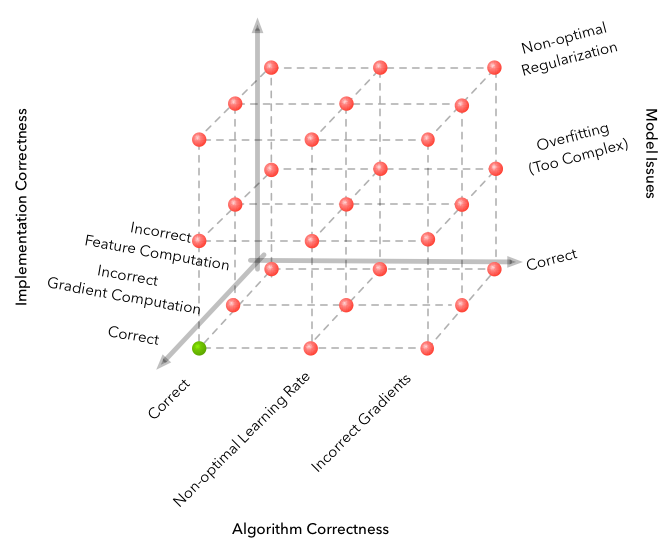
RL algorithms fall along a continuum, where they get to assume more or less knowledge about the environment they’re in. The broadest category, model-free RL, is almost the same as black-box optimization. These methods are only allowed to assume they are in an MDP. Otherwise, they are given nothing else. The agent is simply told that this gives +1 reward, this doesn’t, and it has to learn the rest on its own. And like black-box optimization, the problem is that anything that gives +1 reward is good, even if the +1 reward isn’t coming for the right reasons.
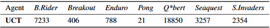
A classic non-RL example is the time someone applied genetic algorithms to circuit design, and got a circuit where an unconnected logic gate was necessary to the final design.
The gray cells are required to get correct behavior, including the one in the top-left corner, even though it’s connected to nothing. From “An Evolved Circuit, Intrinsic in Silicon, Entwined with Physics”
For a more recent example, see this 2017 blog post from Salesforce. Their goal is text summarization. Their baseline model is trained with supervised learning, then evaluated with an automated metric called ROUGE. ROUGE is non-differentiable, but RL can deal with non-differentiable rewards, so they tried applying RL to optimize ROUGE directly. This gives high ROUGE (hooray!), but it doesn’t actually give good summaries. Here’s an example.
Button was denied his 100th race for McLaren after an ERS prevented him from making it to the start-line. It capped a miserable weekend for the Briton. Button has out-qualified. Finished ahead of Nico Rosberg at Bahrain. Lewis Hamilton has. In 11 races. . The race. To lead 2,000 laps. . In. . . And.
So, despite the RL model giving the highest ROUGE score…
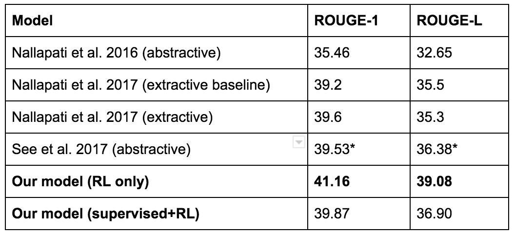
they ended up using a different model instead.
Here’s another fun example. This is Popov et al, 2017, sometimes known as “the Lego stacking paper”. The authors use a distributed version of DDPG to learn a grasping policy. The goal is to grasp the red block, and stack it on top of the blue block.
They got it to work, but they ran into a neat failure case. For the initial lifting motion, reward is given based on how high the red block is. This is defined by the z-coordinate of the bottom face of the block. One of the failure modes was that the policy learned to tip the red block over, instead of picking it up.
Now, clearly this isn’t the intended solution. But RL doesn’t care. From the perspective of reinforcement learning, it got rewarded for flipping a block, so it’s going to keep flipping blocks.
One way to address this is to make the reward sparse, by only giving positive reward after the robot stacks the block. Sometimes, this works, because the sparse reward is learnable. Often, it doesn’t, because the lack of positive reinforcement makes everything too difficult.
The other way to address this is to do careful reward shaping, adding new reward terms and tweaking coefficients of existing ones until the behaviors you want to learn fall out of the RL algorithm. It’s possible to fight RL on this front, but it’s a very unfulfilling fight. On occasion, it’s necessary, but I’ve never felt like I’ve learnt anything by doing it.
For reference, here is one of the reward functions from the Lego stacking paper.
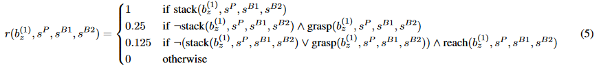
I don’t know how much time was spent designing this reward, but based on the number of terms and the number of different coefficients, I’m going to guess “a lot”.
In talks with other RL researchers, I’ve heard several anecdotes about the novel behavior they’ve seen from improperly defined rewards.
-
A coworker is teaching an agent to navigate a room. The episode terminates if the agent walks out of bounds. He didn’t add any penalty if the episode terminates this way. The final policy learned to be suicidal, because negative reward was plentiful, positive reward was too hard to achieve, and a quick death ending in 0 reward was preferable to a long life that risked negative reward.
-
A friend is training a simulated robot arm to reach towards a point above a table. It turns out the point was defined with respect to the table, and the table wasn’t anchored to anything. The policy learned to slam the table really hard, making the table fall over, which moved the target point too. The target point just so happened to fall next to the end of the arm.
-
A researcher gives a talk about using RL to train a simulated robot hand to pick up a hammer and hammer in a nail. Initially, the reward was defined by how far the nail was pushed into the hole. Instead of picking up the hammer, the robot used its own limbs to punch the nail in. So, they added a reward term to encourage picking up the hammer, and retrained the policy. They got the policy to pick up the hammer…but then it threw the hammer at the nail instead of actually using it.
Admittedly, these are all secondhand accounts, and I haven’t seen videos of any of these behaviors. However, none of it sounds implausible to me. I’ve been burned by RL too many times to believe otherwise.
I know people who like to tell stories about paperclip optimizers. I get it, I really do. But honestly, I’m sick of hearing those stories, because they always speculate up some superhuman misaligned AGI to create a just-so story. There’s no reason to speculate that far when present-day examples happen all the time.
Even Given a Good Reward, Local Optima Can Be Hard To Escape
The previous examples of RL are sometimes called “reward hacking”. To me, this implies a clever, out-of-the-box solution that gives more reward than the intended answer of the reward function designer.
Reward hacking is the exception. The much more common case is a poor local optima that comes from getting the exploration-exploitation trade-off wrong.
Here’s one of my favorite videos. This is an implementation of Normalized Advantage Function, learning on the HalfCheetah environment.
From an outside perspective, this is really, really dumb. But we can only say it’s dumb because we can see the 3rd person view, and have a bunch of prebuilt knowledge that tells us running on your feet is better. RL doesn’t know this! It sees a state vector, it sends action vectors, and it knows it’s getting some positive reward. That’s it.
Here’s my best guess for what happened during learning.
- In random exploration, the policy found falling forward was better than standing still.
- It did so enough to “burn in” that behavior, so now it’s falling forward consistently.
- After falling forward, the policy learned that if it does a one-time application of a lot of force, it’ll do a backflip that gives a bit more reward.
- It explored the backflip enough to become confident this was a good idea, and now backflipping is burned into the policy.
- Once the policy is backflipping consistently, which is easier for the policy: learning to right itself and then run “the standard way”, or learning or figuring out how to move forward while lying on its back? I would guess the latter.
It’s very funny, but it definitely isn’t what I wanted the robot to do.
Here’s another failed run, this time on the Reacher environment.
In this run, the initial random weights tended to output highly positive or highly negative action outputs. This makes most of the actions output the maximum or minimum acceleration possible. It’s really easy to spin super fast: just output high magnitude forces at every joint. Once the robot gets going, it’s hard to deviate from this policy in a meaningful way - to deviate, you have to take several exploration steps to stop the rampant spinning. It’s certainly possible, but in this run, it didn’t happen.
These are both cases of the classic exploration-exploitation problem that has dogged reinforcement learning since time immemorial. Your data comes from your current policy. If your current policy explores too much you get junk data and learn nothing. Exploit too much and you burn-in behaviors that aren’t optimal.
There are several intuitively pleasing ideas for addressing this - intrinsic motivation, curiosity-driven exploration, count-based exploration, and so forth. Many of these approaches were first proposed in the 1980s or earlier, and several of them have been revisited with deep learning models. However, as far as I know, none of them work consistently across all environments. Sometimes they help, sometimes they don’t. It would be nice if there was an exploration trick that worked everywhere, but I’m skeptical a silver bullet of that caliber will be discovered anytime soon. Not because people aren’t trying, but because exploration-exploitation is really, really, really, really, really hard. To quote Wikipedia,
Originally considered by Allied scientists in World War II, it proved so intractable that, according to Peter Whittle, the problem was proposed to be dropped over Germany so that German scientists could also waste their time on it.
(Reference: Q-Learning for Bandit Problems, Duff 1995)
I’ve taken to imagining deep RL as a demon that’s deliberately misinterpreting your reward and actively searching for the laziest possible local optima. It’s a bit ridiculous, but I’ve found it’s actually a productive mindset to have.
Even When Deep RL Works, It May Just Be Overfitting to Weird Patterns In the Environment
Deep RL is popular because it’s the only area in ML where it’s socially acceptable to train on the test set.
The upside of reinforcement learning is that if you want to do well in an environment, you’re free to overfit like crazy. The downside is that if you want to generalize to any other environment, you’re probably going to do poorly, because you overfit like crazy.
DQN can solve a lot of the Atari games, but it does so by focusing all of learning on a single goal - getting really good at one game. The final model won’t generalize to other games, because it hasn’t been trained that way. You can finetune a learned DQN to a new Atari game (see Progressive Neural Networks (Rusu et al, 2016)), but there’s no guarantee it’ll transfer and people usually don’t expect it to transfer. It’s not the wild success people see from pretrained ImageNet features.
To forestall some obvious comments: yes, in principle, training on a wide distribution of environments should make these issues go away. In some cases, you get such a distribution for free. An example is navigation, where you can sample goal locations randomly, and use universal value functions to generalize. (See Universal Value Function Approximators, Schaul et al, ICML 2015.) I find this work very promising, and I give more examples of this work later. However, I don’t think the generalization capabilities of deep RL are strong enough to handle a diverse set of tasks yet. Perception has gotten a lot better, but deep RL has yet to have its “ImageNet for control” moment. OpenAI Universe tried to spark this, but from what I heard, it was too difficult to solve, so not much got done.
Until we have that kind of generalization moment, we’re stuck with policies that can be surprisingly narrow in scope. As an example of this (and as an opportunity to poke fun at some of my own work), consider Can Deep RL Solve Erdos-Selfridge-Spencer Games? (Raghu et al, 2017). We studied a toy 2-player combinatorial game, where there’s a closed-form analytic solution for optimal play. In one of our first experiments, we fixed player 1’s behavior, then trained player 2 with RL. By doing this, you can treat player 1’s actions as part of the environment. By training player 2 against the optimal player 1, we showed RL could reach high performance. But when we deployed the same policy against a non-optimal player 1, its performance dropped, because it didn’t generalize to non-optimal opponents.
Lanctot et al, NIPS 2017 showed a similar result. Here, there are two agents playing laser tag. The agents are trained with multiagent reinforcement learning. To test generalization, they run the training with 5 random seeds. Here’s a video of agents that have been trained against one another.
As you can see, they learn to move towards and shoot each other. Then, they took player 1 from one experiment, and pitted it against player 2 from a different experiment. If the learned policies generalize, we should see similar behavior.
Spoiler alert: they don’t.
This seems to be a running theme in multiagent RL. When agents are trained against one another, a kind of co-evolution happens. The agents get really good at beating each other, but when they get deployed against an unseen player, performance drops. I’d also like to point out that the only difference between these videos is the random seed. Same learning algorithm, same hyperparameters. The diverging behavior is purely from randomness in initial conditions.
That being said, there are some neat results from competitive self-play environments that seem to contradict this. OpenAI has a nice blog post of some of their work in this space. Self-play is also an important part of both AlphaGo and AlphaZero. My intuition is that if your agents are learning at the same pace, they can continually challenge each other and speed up each other’s learning, but if one of them learns much faster, it exploits the weaker player too much and overfits. As you relax from symmetric self-play to general multiagent settings, it gets harder to ensure learning happens at the same speed.
Even Ignoring Generalization Issues, The Final Results Can be Unstable and Hard to Reproduce
Almost every ML algorithm has hyperparameters, which influence the behavior of the learning system. Often, these are picked by hand, or by random search.
Supervised learning is stable. Fixed dataset, ground truth targets. If you change the hyperparameters a little bit, your performance won’t change that much. Not all hyperparameters perform well, but with all the empirical tricks discovered over the years, many hyperparams will show signs of life during training. These signs of life are super important, because they tell you that you’re on the right track, you’re doing something reasonable, and it’s worth investing more time.
Currently, deep RL isn’t stable at all, and it’s just hugely annoying for research.
When I started working at Google Brain, one of the first things I did was implement the algorithm from the Normalized Advantage Function paper. I figured it would only take me about 2-3 weeks. I had several things going for me: some familiarity with Theano (which transferred to TensorFlow well), some deep RL experience, and the first author of the NAF paper was interning at Brain, so I could bug him with questions.
It ended up taking me 6 weeks to reproduce results, thanks to several software bugs. The question is, why did it take so long to find these bugs?
To answer this, let’s consider the simplest continuous control task in OpenAI Gym: the Pendulum task. In this task, there’s a pendulum, anchored at a point, with gravity acting on the pendulum. The input state is 3-dimensional. The action space is 1-dimensional, the amount of torque to apply. The goal is to balance the pendulum perfectly straight up.
This is a tiny problem, and it’s made even easier by a well shaped reward. Reward is defined by the angle of the pendulum. Actions bringing the pendulum closer to the vertical not only give reward, they give increasing reward. The reward landscape is basically concave.
Below is a video of a policy that mostly works. Although the policy doesn’t balance straight up, it outputs the exact torque needed to counteract gravity.
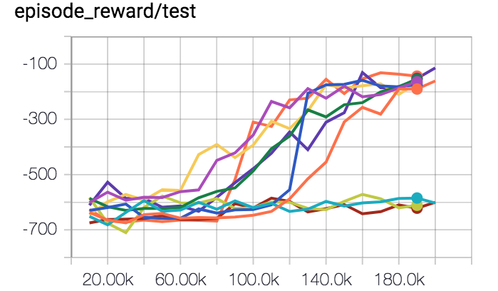
Here is a plot of performance, after I fixed all the bugs. Each line is the reward curve from one of 10 independent runs. Same hyperparameters, the only difference is the random seed.
Seven of these runs worked. Three of these runs didn’t. A 30% failure rate counts as working. Here’s another plot from some published work, “Variational Information Maximizing Exploration” (Houthooft et al, NIPS 2016). The environment is HalfCheetah. The reward is modified to be sparser, but the details aren’t too important. The y-axis is episode reward, the x-axis is number of timesteps, and the algorithm used is TRPO.
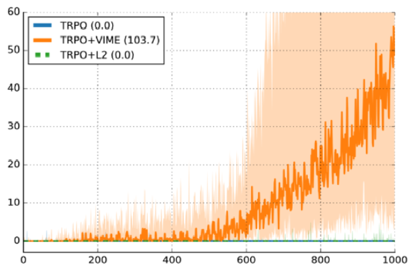
The dark line is the median performance over 10 random seeds, and the shaded region is the 25th to 75th percentile. Don’t get me wrong, this plot is a good argument in favor of VIME. But on the other hand, the 25th percentile line is really close to 0 reward. That means about 25% of runs are failing, just because of random seed.
Look, there’s variance in supervised learning too, but it’s rarely this bad. If my supervised learning code failed to beat random chance 30% of the time, I’d have super high confidence there was a bug in data loading or training. If my reinforcement learning code does no better than random, I have no idea if it’s a bug, if my hyperparameters are bad, or if I simply got unlucky.
This picture is from “Why is Machine Learning ‘Hard’?”. The core thesis is that machine learning adds more dimensions to your space of failure cases, which exponentially increases the number of ways you can fail. Deep RL adds a new dimension: random chance. And the only way you can address random chance is by throwing enough experiments at the problem to drown out the noise.
When your training algorithm is both sample inefficient and unstable, it heavily slows down your rate of productive research. Maybe it only takes 1 million steps. But when you multiply that by 5 random seeds, and then multiply that with hyperparam tuning, you need an exploding amount of compute to test hypotheses effectively.
If it makes you feel any better, I’ve been doing this for a while and it took me last ~6 weeks to get a from-scratch policy gradients implementation to work 50% of the time on a bunch of RL problems. And I also have a GPU cluster available to me, and a number of friends I get lunch with every day who’ve been in the area for the last few years.
Also, what we know about good CNN design from supervised learning land doesn’t seem to apply to reinforcement learning land, because you’re mostly bottlenecked by credit assignment / supervision bitrate, not by a lack of a powerful representation. Your ResNets, batchnorms, or very deep networks have no power here.
[Supervised learning] wants to work. Even if you screw something up you’ll usually get something non-random back. RL must be forced to work. If you screw something up or don’t tune something well enough you’re exceedingly likely to get a policy that is even worse than random. And even if it’s all well tuned you’ll get a bad policy 30% of the time, just because.
Long story short your failure is more due to the difficulty of deep RL, and much less due to the difficulty of “designing neural networks”.
Hacker News comment from Andrej Karpathy, back when he was at OpenAI
Instability to random seed is like a canary in a coal mine. If pure randomness is enough to lead to this much variance between runs, imagine how much an actual difference in the code could make.
Luckily, we don’t have to imagine, because this was inspected by the paper “Deep Reinforcement Learning That Matters” (Henderson et al, AAAI 2018). Among its conclusions are:
- Multiplying the reward by a constant can cause significant differences in performance.
- Five random seeds (a common reporting metric) may not be enough to argue significant results, since with careful selection you can get non-overlapping confidence intervals.
- Different implementations of the same algorithm have different performance on the same task, even when the same hyperparameters are used.
My theory is that RL is very sensitive to both your initialization and to the dynamics of your training process, because your data is always collected online and the only supervision you get is a single scalar for reward. A policy that randomly stumbles onto good training examples will bootstrap itself much faster than a policy that doesn’t. A policy that fails to discover good training examples in time will collapse towards learning nothing at all, as it becomes more confident that any deviation it tries will fail.
But What About All The Great Things Deep RL Has Done For Us?
Deep reinforcement learning has certainly done some very cool things. DQN is old news now, but was absolutely nuts at the time. A single model was able to learn directly from raw pixels, without tuning for each game individually. And AlphaGo and AlphaZero continue to be very impressive achievements.
However, outside of these successes, it’s hard to find cases where deep RL has created practical real world value.
I tried to think of real-world, productionized uses of deep RL, and it was surprisingly difficult. I expected to find something in recommendation systems, but I believe those are still dominated by collaborative filtering and contextual bandits.
In the end, the best I could find were two Google projects: reducing data center power usage, and the recently announced AutoML Vision effort. Jack Clark from OpenAI tweeted a similar request and found a similar conclusion. (The tweet is from last year, before AutoML was announced.)
I know Audi’s doing something with deep RL, since they demoed a self-driving RC car at NIPS and said it used deep RL. I know there’s some neat work optimizing device placement for large Tensorflow graphs (Mirhoseini et al, ICML 2017). Salesforce has their text summarization model, which worked if you massaged the RL carefully enough. Finance companies are surely experimenting with RL as we speak, but so far there’s no definitive proof. (Of course, finance companies have reasons to be cagey about how they play the market, so perhaps the evidence there is never going to be strong.) Facebook’s been doing some neat work with deep RL for chatbots and conversation. Every Internet company ever has probably thought about adding RL to their ad-serving model, but if anyone’s done it, they’ve kept quiet about it.
The way I see it, either deep RL is still a research topic that isn’t robust enough for widespread use, or it’s usable and the people who’ve gotten it to work aren’t publicizing it. I think the former is more likely.
If you came to me with an image classification problem, I’d point you to pretrained ImageNet models, and they’d probably do great. We’re in a world where the people behind Silicon Valley can build a real Not Hotdog app as a joke. I have trouble seeing the same happen with deep RL.
Given Current Limitations, When Could Deep RL Work For Me?
A priori, it’s really hard to say. The problem with trying to solve everything with RL is that you’re trying to solve several very different environments with the same approach. It’s only natural that it won’t work all the time.
That being said, we can draw conclusions from the current list of deep reinforcement learning successes. These are projects where deep RL either learns some qualitatively impressive behavior, or it learns something better than comparable prior work. (Admittedly, this is a very subjective criteria.)
Here’s my list so far.
- Things mentioned in the previous sections: DQN, AlphaGo, AlphaZero, the parkour bot, reducing power center usage, and AutoML with Neural Architecture Search.
- OpenAI’s Dota 2 1v1 Shadow Fiend bot, which beat top pro players in a simplified duel setting.
- A Super Smash Brothers Melee bot that can beat pro players at 1v1 Falcon dittos. (Firoiu et al, 2017).
(A quick aside: machine learning recently beat pro players at no-limit heads up Texas Hold’Em. This was done by both Libratus (Brown et al, IJCAI 2017) and DeepStack (Moravčík et al, 2017). I’ve talked to a few people who believed this was done with deep RL. They’re both very cool, but they don’t use deep RL. They use counterfactual regret minimization and clever iterative solving of subgames.)
From this list, we can identify common properties that make learning easier. None of the properties below are required for learning, but satisfying more of them is definitively better.
-
It is easy to generate near unbounded amounts of experience. It should be clear why this helps. The more data you have, the easier the learning problem is. This applies to Atari, Go, Chess, Shogi, and the simulated environments for the parkour bot. It likely applies to the power center project too, because in prior work (Gao, 2014), it was shown that neural nets can predict energy efficiency with high accuracy. That’s exactly the kind of simulated model you’d want for training an RL system.
It might apply to the Dota 2 and SSBM work, but it depends on the throughput of how quickly the games can be run, and how many machines were available to run them.
-
The problem is simplified into an easier form. One of the common errors I’ve seen in deep RL is to dream too big. Reinforcement learning can do anything! That doesn’t mean you have to do everything at once.
The OpenAI Dota 2 bot only played the early game, only played Shadow Fiend against Shadow Fiend in a 1v1 laning setting, used hardcoded item builds, and presumably called the Dota 2 API to avoid having to solve perception. The SSBM bot acheived superhuman performance, but it was only in 1v1 games, with Captain Falcon only, on Battlefield only, in an infinite time match.
This isn’t a dig at either bot. Why work on a hard problem when you don’t even know the easier one is solvable? The broad trend of all research is to demonstrate the smallest proof-of-concept first and generalize it later. OpenAI is extending their Dota 2 work, and there’s ongoing work to extend the SSBM bot to other characters.
-
There is a way to introduce self-play into learning. This is a component of AlphaGo, AlphaZero, the Dota 2 Shadow Fiend bot, and the SSBM Falcon bot. I should note that by self-play, I mean exactly the setting where the game is competitive, and both players can be controlled by the same agent. So far, that setting seems to have the most stable and well-performing behavior.
-
There’s a clean way to define a learnable, ungameable reward. Two player games have this: +1 for a win, -1 for a loss. The original neural architecture search paper from Zoph et al, ICLR 2017 had this: validation accuracy of the trained model. Any time you introduce reward shaping, you introduce a chance for learning a non-optimal policy that optimizes the wrong objective.
If you’re interested in further reading on what makes a good reward, a good search term is “proper scoring rule”. See this Terrence Tao blog post for an approachable example.
As for learnability, I have no advice besides trying it out to see if it works.
-
If the reward has to be shaped, it should at least be rich. In Dota 2, reward can come from last hits (triggers after every monster kill by either player), and health (triggers after every attack or skill that hits a target.) These reward signals come quick and often. For the SSBM bot, reward can be given for damage dealt and taken, which gives signal for every attack that successfully lands. The shorter the delay between action and consequence, the faster the feedback loop gets closed, and the easier it is for reinforcement learning to figure out a path to high reward.
A Case Study: Neural Architecture Search
We can combine a few of the principles to analyze the success of Neural Architecture Search. According to the initial ICLR 2017 version, after 12800 examples, deep RL was able to design state-of-the art neural net architectures. Admittedly, each example required training a neural net to convergence, but this is still very sample efficient.
As mentioned above, the reward is validation accuracy. This is a very rich reward signal - if a neural net design decision only increases accuracy from 70% to 71%, RL will still pick up on this. Additionally, there’s evidence that hyperparameters in deep learning are close to linearly independent. (This was empirically shown in Hyperparameter Optimization: A Spectral Approach (Hazan et al, 2017) - a summary by me is here if interested.) NAS isn’t exactly tuning hyperparameters, but I think it’s reasonable that neural net design decisions would act similarly. This is good news for learning, because the correlations between decision and performance are strong. Finally, not only is the reward rich, it’s actually what we care about when we train models.
The combination of all these points helps me understand why it “only” takes about 12800 trained networks to learn a better one, compared to the millions of examples needed in other environments. Several parts of the problem are all pushing in RL’s favor.
Overall, success stories this strong are still the exception, not the rule. Many things have to go right for reinforcement learning to be a plausible solution, and even then, it’s not a free ride to make that solution happen.
In short: deep RL is currently not a plug-and-play technology.
Looking to The Future
There’s an old saying - every researcher learns how to hate their area of study. The trick is that researchers will press on despite this, because they like the problems too much.
That’s roughly how I feel about deep reinforcement learning. Despite my reservations, I think people absolutely should be throwing RL at different problems, including ones where it probably shouldn’t work. How else are we supposed to make RL better?
I see no reason why deep RL couldn’t work, given more time. Several very interesting things are going to happen when deep RL is robust enough for wider use. The question is how it’ll get there.
Below, I’ve listed some futures I find plausible. For the futures based on further research, I’ve provided citations to relevant papers in those research areas.
Local optima are good enough: It would be very arrogant to claim humans are globally optimal at anything. I would guess we’re juuuuust good enough to get to civilization stage, compared to any other species. In the same vein, an RL solution doesn’t have to achieve a global optima, as long as its local optima is better than the human baseline.
Hardware solves everything: I know some people who believe that the most influential thing that can be done for AI is simply scaling up hardware. Personally, I’m skeptical that hardware will fix everything, but it’s certainly going to be important. The faster you can run things, the less you care about sample inefficiency, and the easier it is to brute-force your way past exploration problems.
Add more learning signal: Sparse rewards are hard to learn because you get very little information about what thing help you. It’s possible we can either hallucinate positive rewards (Hindsight Experience Replay, Andrychowicz et al, NIPS 2017), define auxiliary tasks (UNREAL, Jaderberg et al, NIPS 2016), or bootstrap with self-supervised learning to build good world model. Adding more cherries to the cake, so to speak.
Model-based learning unlocks sample efficiency: Here’s how I describe model-based RL: “Everyone wants to do it, not many people know how.” In principle, a good model fixes a bunch of problems. As seen in AlphaGo, having a model at all makes it much easier to learn a good solution. Good world models will transfer well to new tasks, and rollouts of the world model let you imagine new experience. From what I’ve seen, model-based approaches use fewer samples as well.
The problem is that learning good models is hard. My impression is that low-dimensional state models work sometimes, and image models are usually too hard. But, if this gets easier, some interesting things could happen.
Dyna (Sutton, 1991) and Dyna-2 (Silver et al., ICML 2008) are classical papers in this space. For papers combining model-based learning with deep nets, I would recommend a few recent papers from the Berkeley robotics labs: Neural Network Dynamics for Model-Based Deep RL with Model-Free Fine-Tuning (Nagabandi et al, 2017, Self-Supervised Visual Planning with Temporal Skip Connections (Ebert et al, CoRL 2017), Combining Model-Based and Model-Free Updates for Trajectory-Centric Reinforcement Learning (Chebotar et al, ICML 2017). Deep Spatial Autoencoders for Visuomotor Learning (Finn et al, ICRA 2016), and Guided Policy Search (Levine et al, JMLR 2016).
Use reinforcement learning just as the fine-tuning step: The first AlphaGo paper started with supervised learning, and then did RL fine-tuning on top of it. This is a nice recipe, since it lets you use a faster-but-less-powerful method to speed up initial learning. It’s worked in other contexts - see Sequence Tutor (Jaques et al, ICML 2017). You can view this as starting the RL process with a reasonable prior, instead of a random one, where the problem of learning the prior is offloaded to some other approach.
Reward functions could be learnable: The promise of ML is that we can use data to learn things that are better than human design. If reward function design is so hard, Why not apply this to learn better reward functions? Imitation learning and inverse reinforcement learning are both rich fields that have shown reward functions can be implicitly defined by human demonstrations or human ratings.
For famous papers in inverse RL and imitation learning, see Algorithms for Inverse Reinforcement Learning (Ng and Russell, ICML 2000), Apprenticeship Learning via Inverse Reinforcement Learning (Abbeel and Ng, ICML 2004), and DAgger (Ross, Gordon, and Bagnell, AISTATS 2011).
For recent work scaling these ideas to deep learning, see Guided Cost Learning (Finn et al, ICML 2016), Time-Constrastive Networks (Sermanet et al, 2017), and Learning From Human Preferences (Christiano et al, NIPS 2017). (The Human Preferences paper in particular showed that a reward learned from human ratings was actually better-shaped for learning than the original hardcoded reward, which is a neat practical result.)
For longer term work that doesn’t use deep learning, I liked Inverse Reward Design (Hadfield-Menell et al, NIPS 2017) and Learning Robot Objectives from Physical Human Interaction (Bajcsy et al, CoRL 2017).
Transfer learning saves the day: The promise of transfer learning is that you can leverage knowledge from previous tasks to speed up learning of new ones. I think this is absolutely the future, when task learning is robust enough to solve several disparate tasks. It’s hard to do transfer learning if you can’t learn at all, and given task A and task B, it can be very hard to predict whether A transfers to B. In my experience, it’s either super obvious, or super unclear, and even the super obvious cases aren’t trivial to get working.
Universal Value Function Approximators (Schaul et al, ICML 2015), Distral (Whye Teh et al, NIPS 2017), and Overcoming Catastrophic Forgetting (Kirkpatrick et al, PNAS 2017) are recent works in this direction. For older work, consider reading Horde (Sutton et al, AAMAS 2011).
Robotics in particular has had lots of progress in sim-to-real transfer (transfer learning between a simulated version of a task and the real task). See Domain Randomization (Tobin et al, IROS 2017), Sim-to-Real Robot Learning with Progressive Nets (Rusu et al, CoRL 2017), and GraspGAN (Bousmalis et al, 2017). (Disclaimer: I worked on GraspGAN.)
Good priors could heavily reduce learning time: This is closely tied to several of the previous points. In one view, transfer learning is about using past experience to build a good prior for learning other tasks. RL algorithms are designed to apply to any Markov Decision Process, which is where the pain of generality comes in. If we accept that our solutions will only perform well on a small section of environments, we should be able to leverage shared structure to solve those environments in an efficient way.
One point Pieter Abbeel likes to mention in his talks is that deep RL only needs to solve tasks that we expect to need in the real world. I agree it makes a lot of sense. There should exist a real-world prior that lets us quickly learn new real-world tasks, at the cost of slower learning on non-realistic tasks, but that’s a perfectly acceptable trade-off.
The difficulty is that such a real-world prior will be very hard to design. However, I think there’s a good chance it won’t be impossible. Personally, I’m excited by the recent work in metalearning, since it provides a data-driven way to generate reasonable priors. For example, if I wanted to use RL to do warehouse navigation, I’d get pretty curious about using metalearning to learn a good navigation prior, and then fine-tuning the prior for the specific warehouse the robot will be deployed in. This very much seems like the future, and the question is whether metalearning will get there or not.
A summary of recent learning-to-learn work can be found in this post from BAIR (Berkeley AI Research).
Harder environments could paradoxically be easier: One of the big lessons from the DeepMind parkour paper is that if you make your task very difficult by adding several task variations, you can actually make the learning easier, because the policy cannot overfit to any one setting without losing performance on all the other settings. We’ve seen a similar thing in the domain randomization papers, and even back to ImageNet: models trained on ImageNet will generalize way better than ones trained on CIFAR-100. As I said above, maybe we’re just an “ImageNet for control” away from making RL considerably more generic.
Environment wise, there are a lot of options. OpenAI Gym easily has the most traction, but there’s also the Arcade Learning Environment, Roboschool, DeepMind Lab, the DeepMind Control Suite, and ELF.
Finally, although it’s unsatisfying from a research perspective, the empirical issues of deep RL may not matter for practical purposes. As a hypothetical example, suppose a finance company is using deep RL. They train a trading agent based on past data from the US stock market, using 3 random seeds. In live A/B testing, one gives 2% less revenue, one performs the same, and one gives 2% more revenue. In that hypothetical, reproducibility doesn’t matter - you deploy the model with 2% more revenue and celebrate. Similarly, it doesn’t matter that the trading agent may only perform well in the United States - if it generalizes poorly to the worldwide market, just don’t deploy it there. There is a large gap between doing something extraordinary and making that extraordinary success reproducible, and maybe it’s worth focusing on the former first.
Where We Are Now
In many ways, I find myself annoyed with the current state of deep RL. And yet, it’s attracted some of the strongest research interest I’ve ever seen. My feelings are best summarized by a mindset Andrew Ng mentioned in his Nuts and Bolts of Applying Deep Learning talk - a lot of short-term pessimism, balanced by even more long-term optimism. Deep RL is a bit messy right now, but I still believe in where it could be.
That being said, the next time someone asks me whether reinforcement learning can solve their problem, I’m still going to tell them that no, it can’t. But I’ll also tell them to ask me again in a few years. By then, maybe it can.
* * *
This post went through a lot of revision. Thanks go to following people for reading earlier drafts: Daniel Abolafia, Kumar Krishna Agrawal, Surya Bhupatiraju, Jared Quincy Davis, Ashley Edwards, Peter Gao, Julian Ibarz, Sherjil Ozair, Vitchyr Pong, Alex Ray, and Kelvin Xu. There were several more reviewers who I’m crediting anonymously - thanks for all the feedback.
-
-
MIT Mystery Hunt 2018
CommentsI plan to edit in puzzle links later.
After going in-person for the past 2 Hunts, I decided not to fly-in for the 2018 Hunt. The short explanation is that I always procrastinate on flights, and at the time I needed to make a decision, work was very, very busy. There were several Code Red, “implement this or nothing is possible” issues.
The issue wasn’t that I didn’t have time. It was that I’d have to take days off on short notice, which would have thrown a bunch of time estimate off. If I had planned Hunt ahead of time, and made sure everyone knew I would be out for certain days, I would have flown in. Lesson learned: hobbies don’t just fall into your life, you make time for your hobbies.
I hunted with ✈✈✈ Galactic Trendsetters ✈✈✈ again. I suppose at this point, it’s my home team, thanks to connections from the high school math contest network.
If you want to avoid spoilers, you should stop reading now.
* * *
Let’s start with broad, overarching feelings about Hunt.
I think Hunt was pretty good! I was worried that a team would finish somewhat quickly, given the warning that Hunt would be shorter than previous years, and that it would be best if your team wasn’t too large. My expectation was that it would be fewer puzzles, team sizes wouldn’t change, the winning team would solve Hunt pretty quickly, and then the rest of us would get there along the way. The initial Emotions round did nothing to disprove this. It turned out that the Island puzzles were a lot harder, big teams had decided to split ahead of Hunt, this was still MIT Mystery Hunt and it was still going to be A Journey.
Number of puzzles isn’t the only metric that matters in Hunt. Unlock structure matters too. If it’s harder to unlock a bunch of puzzles, it’s harder to parallelize solving, which slows down Hunt and leads to bottlenecking behavior. The easy puzzles get solved instantly, leaving just the hard ones. It’s especially bad for large teams, because the odds you get to see a puzzle before it gets solved just gets vanishingly small.
On the flip side, if it’s too easy to unlock a ton of puzzles, then small teams can get overwhelmed, and big teams just steamroll everything. It’s all a bunch of trade-offs.
Galactic reported 60 people for the scavenger hunt this year, and it definitely felt like we were gated on unlocks. This was especially strong in the Games round, which was our first island. The unlock structure was linear, until you unlocked a puzzle close to the center. It quickly became clear that if we got stuck on any single puzzle, it would potentially block unlocks for a ton of other puzzles. And in fact, that’s what happened for us: both The Year’s Hardest Crossword and Sports Radio were stuck for a while, so we had to rely entirely on solving the linear puzzles up to All the Right Angles before it felt like we were out of danger. In general, I would have liked to see more redundancy in the unlocks for that round.
I have basically zero complaints about the rest of the Hunt. I really like the art aesthetic of the Pokemon round, especially the way it contrasted with the look of the rest of the Hunt. And all the puzzles felt very fair to me.
On to specific stories!
* * *
In the days leading up to Hunt, I made a bingo generator. It seemed like a cute idea, and the site was entirely static, which made it easy to piggyback off Github pages. Unfortunately, I didn’t get a Bingo. I needed “Puzzle is unsolved by the end of Hunt” to get there, and we self-torpedoed my chances by using our spare Buzzy Bucks to buy solutions to all remaining puzzles.
Most recent Hunts have a free answer system that lets you sweep up unsolved puzzles. I’m not sure a zero-solve puzzle is even possible in a modern Hunt.
This was my 6th Mystery Hunt, and I continue to feel like I’m bad at puzzles. I historically have a bad track record at getting a-has. Here’s my main contributions every hunt.
- Telling people we should read the flavor text.
- Telling people we should read the puzzle title.
- Trying to brute-force puzzles by matching partials to whatever word lists I have, and failing.
- Counting things.
- Looking at metapuzzles early, on the off chance they’re easy to solve with partial info.
- Getting really anal about organizing existing data and explaining current puzzle theories.
The way this works out is that I basically never get to do “hero-solves”, because other people hero-solve faster than I do. I feel more like the grease that gets all the other cogs to keep spinning. But, who knows, maybe I underestimate my solving skills.
I spent my Friday morning to afternoon trying to do work while spectating our progress. This was a terrible idea, because I didn’t do much work, and also didn’t get to work on puzzles. I ended up skipping all of the Emotions round. The extent of my contribution was opening the metas, looking at partial progress, and thinking, “oh yeah that’s definitely right.” For the Fear meta in particular, several people on the team had gotten suspicious when the Health & Safety Quiz was mailed to everybody, and got very suspicious when HQ sent a deliberately vague reply as to whether it was a puzzle or not. So when we saw Fear’s flavor text, we got the idea pretty quickly.
Our unlock order was Games, Sci-Fi, Pokemon, Hacking. The first two were by popular vote. By the time we unlocked the third island, it was 1:30 AM on Saturday. Local people didn’t want to do on-campus puzzles at night, and remote people didn’t want to unlock on-campus puzzles because they wanted to have puzzles to work on. This ended up backfiring a bit, because on Saturday night, the only puzzles open were longstanding Games puzzles and physical puzzles, which left little for people who weren’t interested in either. At least it gave me an excuse to go to bed.
The first puzzle I really looked at was Shift, which was cute. I thought “blue shift, red shift”, but didn’t think much of it. Someone else figured out that “gamma” should be shifted to “delta”, I realized “blue shift, red shift” was actually right, and we cleaned it up from there.
I spent a bunch of time on All The Right Angles. One nice thing about crossword-like puzzles is that you can contribute even if you only figure out a few clues. We got the billiards and substituion gimmick pretty quickly, but had trouble getting SIXTUS to fit in our grid. Eventually, someone figured out that “LOUIS IX isn’t LOUIS 9, it’s LOUI6, the cheeky bastards”. After filling in the grid, we drew the billiard path, and someone joked we should call in EIGHT because the path was a figure eight. That gave people some bad flashbacks to SEVEN WONDERS from last year. Luckily, the answer was not EIGHT.
Walk Across Some Dungeons 2 was fun. I was on it instantly, but I moved to other puzzles when I realized I was bad at Sokoban.
When I saw A Tribute: 2010-2017 get unlocked, I immediately thought, “oh sick, I bet this is the puzzle referencing old Hunts”, and then I looked, and it was a puzzle referencing old Hunts. Validation! I didn’t manage to ID any of the old puzzles, and I didn’t solve any of the segments either, but I tried!
I contributed basically zero to the Sci-Fi round. The only thing I did was throw backsolve attempts at the metas now and then.
In the Pokemon round, the first puzzle I worked on was The Advertiser. We figured out they were all TMs, identified them, and then were told it was a metapuzzle. We solved it with 2 answers.
The first regular puzzle we solved in Pokemon was 33 RPM, so Mix Tape was the puzzle where we discovered the evolution gimmick, which was pretty great.
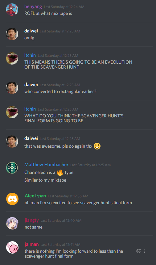
I puzzled with another remote solver, and he was just getting so mad at Mix Tape. It was past midnight, and we had the audio, but the quality was bad. The songs weren’t Shazamable, which was just all kinds of pain. Our image pipeline was “take the spiral image” \(\rightarrow\) “unroll into a rectangular image” \(\rightarrow\) “turn into audio”, but small errors accumulated. In retrospect, reading directly from the raw spiral would have been better.
When Twitch Plays Mystery Hunt came out, I got the impression that literally every local solver started working on it at once. As a remote solver, I unfortunately didn’t get to participate, because all the coordination was getting done in person. I did get to see plenty of memes and copypasta.
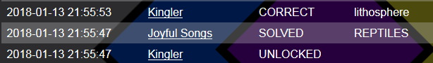
The first “intentionally left blank” puzzle we unlocked was Lycanroc, which confused us for a while. Lycanroc is literally a werewolf, so we thought we had to wait until night for the puzzle to change form. It was a sketchy theory, but we didn’t have anything else. I believe the metameta structure got figured out when somebody noticed the Fire transformation. Once we had that, we got the rest in a matter of minutes. This led to an amusing statistic: our best “solve” time was 6 seconds.
Some people on our team got very, very excited about X Marks the Spot. I didn’t work on it, but as a Euclidean geometry fan, I approve.
The Scouts was the last meta we solved in the Pokemon round. We only solved it after the metameta, when people working on Hacking were looking for things to do. I made a comment about “badges” early on, but it took us a while to discover the puzzle titles were relevant.
When I woke up on Saturday morning, I saw in the chat that Pestered was a Homestuck puzzle. I thought I missed it, but turns out it was stuck on extraction. I didn’t figure the extraction either, and it was the final puzzle we bought. We got tripped up on two things. One, we were certain that we needed to use the DNA pairs of the trolls again, using the zodiac signs to get an ordering. Two, the last page of The Tech from the Thursday before Hunt had horoscopes that looked a lot like puzzle data. Turns out it was a massive, unintentional red herring. I wonder if HQ was confused by our GRYFFINDOR guess.
The first puzzle I worked on in Hacking was Bark Ode. The most amusing part was easily the time where I had to mark a square as ? because I couldn’t figure out if it was a dog or not. I then looked at Voter Fraud, but didn’t do much for it, besides noting it was probably a voting systems puzzle.
I planned to work on Murder at the Asylum, but some local people were solving it at a chalkboard, which didn’t work for remote solvers. So, instead I looked at the Scout meta. Someone else made the key observation that TENDINOPATHIES was likely after a chute and overlapped with EXTEND. There was only one place on the grid that supported that, and with another location guess, we got EXOS as a partial, which was enough to solve the meta. I then worked out constraints on the 3 missing answers, got my work checked, and backsolved Murder at the Asylum before they could forward solve it. Revenge of the remotes!
That ended up being my final contribution to the Hunt. By the time I woke up on Sunday morning, we only had metas, physicals, and abandoned puzzles left. I did some work on drawing out the connectivity graphs for Flee, but that was about it. We did run into one red herring: BIOFUEL TORCH was a tool, BACKUP PLAN sounded like a punt, and EXOSKELETON was a plausible hack, which drove us to think about “Hack, Punt, Tool” for a bit. Somehow, despite never being an MIT student, I still got this reference. The fangs of MIT culture run deep…
I’ll end with a question: what do people think about after finishing a Mystery Hunt?
See you next Hunt! Congrats (and condolences) to Setec.
-
So There I Was, Buying My Little Pony Merchandise in Italy
CommentsFor Thanksgiving, my family went on a trip to Rome. It was pretty cool! There’s something special about visiting a city that is literally thousands of years old. It is one thing to read about the Renaissance, and it is another thing to realize that the sculpture in the town plaza predates the Declaration of Independence by over 300 years, and it’s right there.
The one downside is that although my parents liked the scenery, they weren’t the biggest fans of Italian food. They didn’t dislike it, but, well, let me put it this way: the only restaurant we visited multiple times was a Chinese restaurant.
To be fair, the Chinese restaurant catered to Chinese exchange students, meaning their Chinese food was authentic and actually pretty good. Still, I wasn’t expecting to eat Chinese food in Rome, and I especially wasn’t expecting eating Chinese food multiple times in Rome.
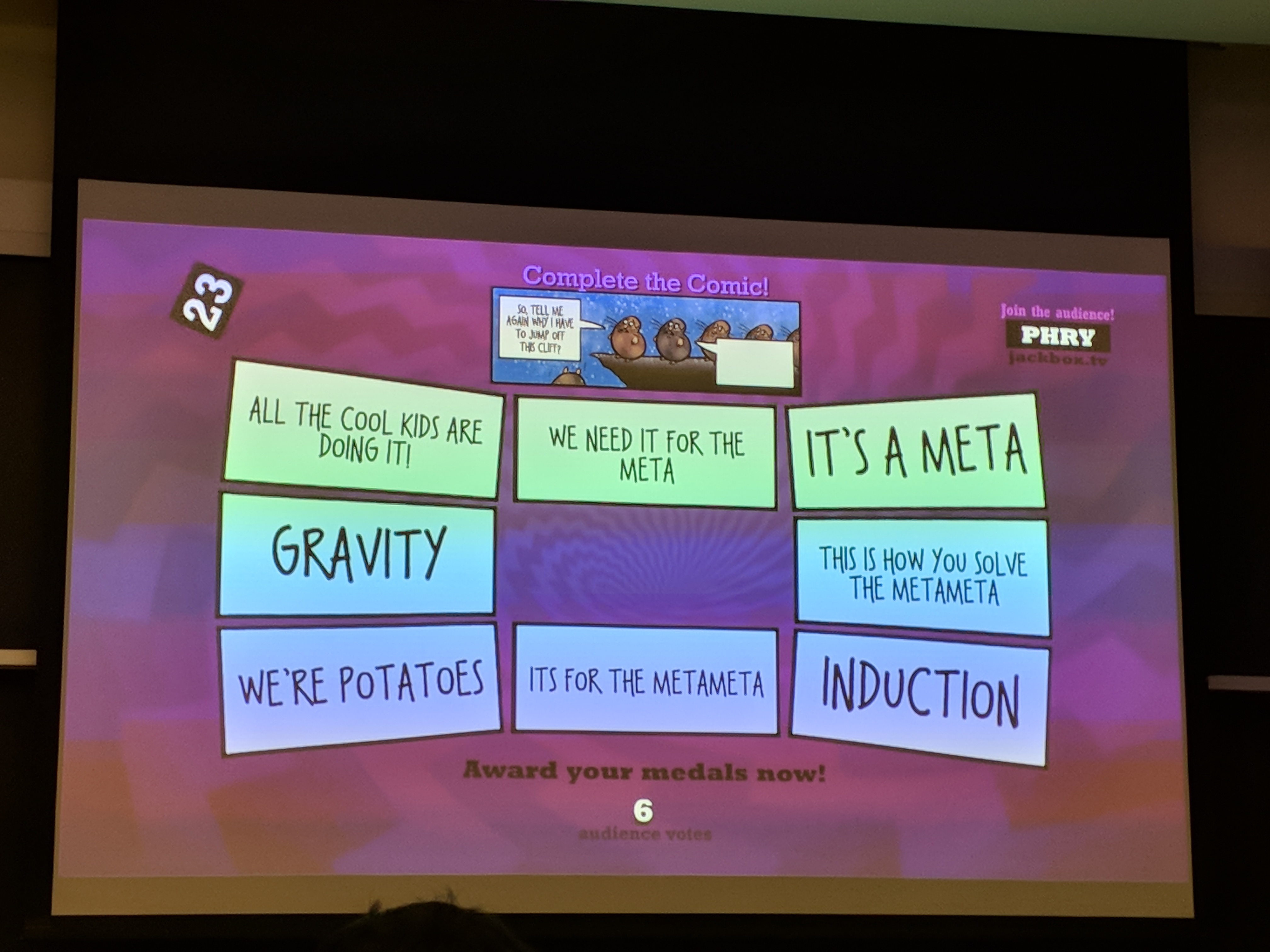
But I digress! During the trip, we visited a supermarket to buy some fruit. While there, a family member pointed out these boxes.

I was against buying it. They argued the following.
- According to the packaging, there was “a surprise inside”.
- It only cost 2 Euros.
- Buying MLP merchandise in Italy is intrinsically funny.
I bought two boxes.
* * *
Let’s take a closer look. The front and back have the same picture, but the two sides are different.


The first thing I noticed was that the character art looked…off, somehow. In what world does Fluttershy wink like that? In what world does Twilight smirk like that. Expression-wise I’m pretty sure neither has made that face in the show, and it feels out-of-character for both of them. Fluttershy seems too reserved for a playful wink. Twilight seems too nice for a knowing smirk.
Rainbow also looked off, and after staring at it a while, I figured out why. Normally her mane hangs over her left eye, but here it hangs over her right.
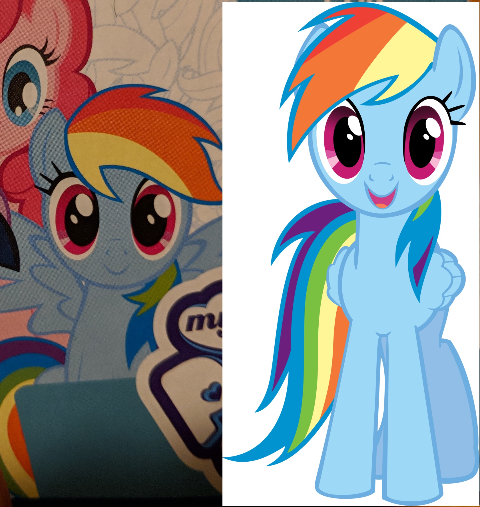
Literally unbuyable. I’m only kind-of joking, actually. Look, here’s my view: fans have the right to call out shitty merchandise. Like, if you’re going to monetize your show, you should at least have your merchandise reflect what your show looks like! Don’t even tell me that the target audience of young girls won’t care. I suspect the target audience does care. One, I believe children are more perceptive than people think. Two, when you’re a kid, you don’t have as much going on in your life, which makes it easy to obsess over the details of your Saturday morning cartoons. The moment they changed Ash Ketchum’s voice actor in Pokemon, I was done with that show.
Take Brave as a case study. The goal of Brave was to create a Disney princess that avoided the gender stereotypes of the old Disney princesses. The movie succeeded. The marketing didn’t.
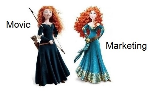
The marketing made Merida slimmer, made her a bit older, removed her bow, and made her hair less curly. Anecdotally, my Facebook feed had a few comments from parents, saying their daughter didn’t like it because “her hair wasn’t as curly”, and “it’s not the same Merida as the movie.” (You can read comments from Brave’s director here, if you’re interested in further ranting.)
The details matter. Don’t mess them up.
* * *
Opening the box produces this.
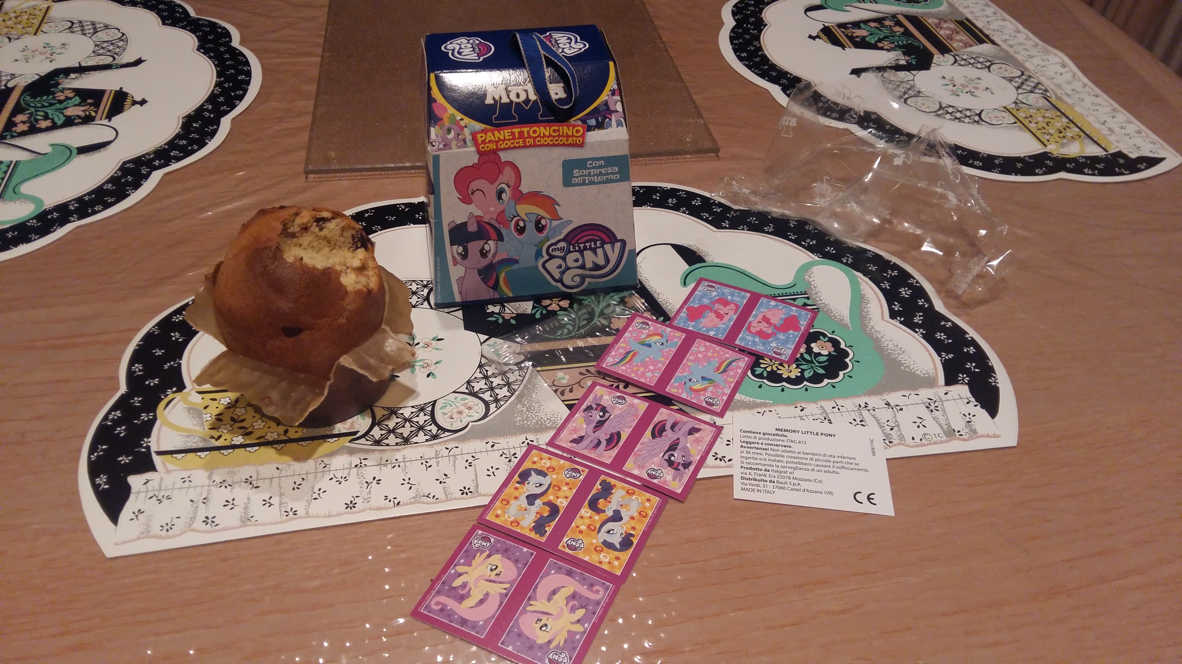
What looked like a chocolate muffin, and a few pony cards. The chocolate muffin…was not that good. Derpy would be ashamed.

Okay, so it’s not actually a muffin. It’s “panettoncino with chocolate chips”, But my headcanon is that if Derpy can make good muffins, she can make good panettoncino too.
Let’s take a closer look at these cards.
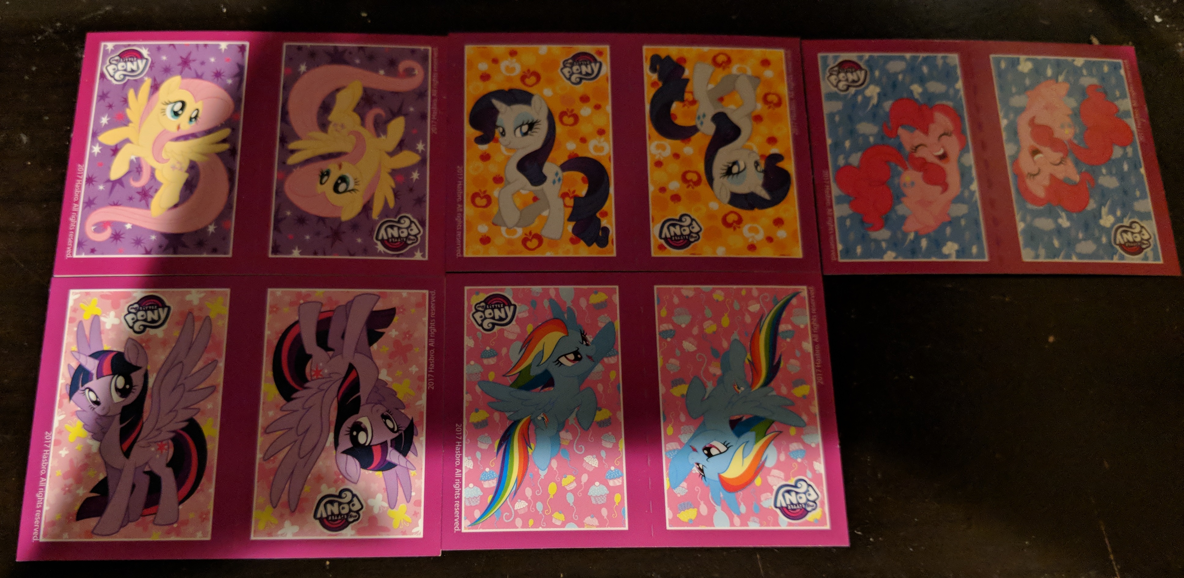
(Card fronts.)
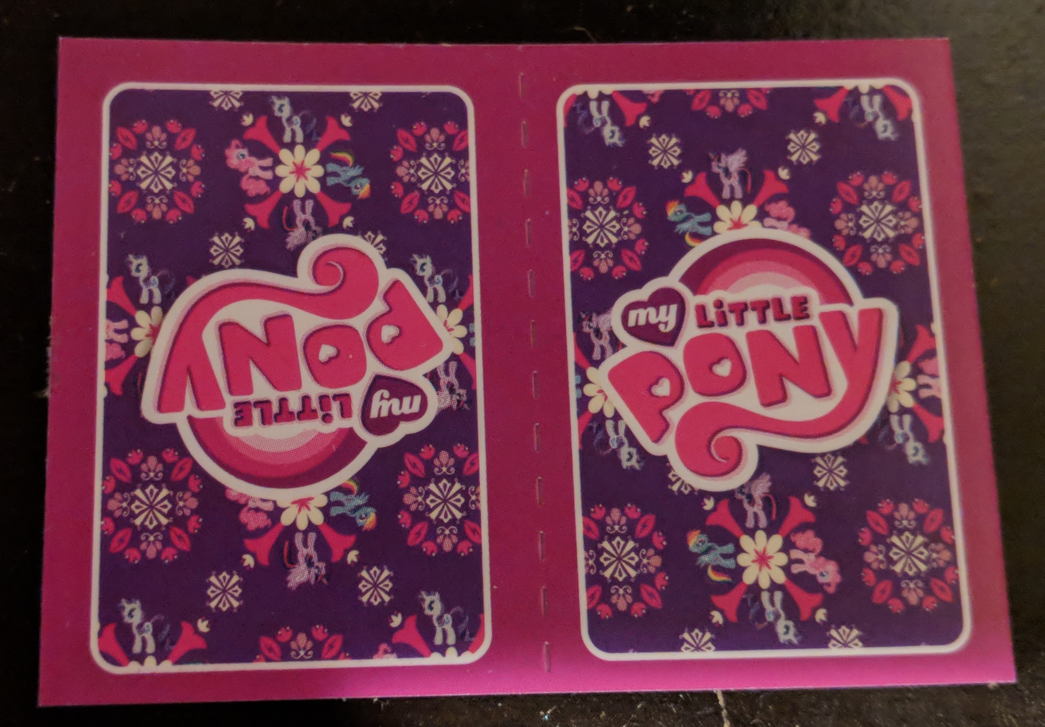
(Card backs. It’s identical for all of them.)
Awwwwww, they’re so cute! I have no issues with the art here. But wait a second, there’s only 5 cards. Isn’t it supposed to be the Mane 6? Where’s Applejack? She’s not on the front. She’s not on the back.
Speaking of which, is Applejack even on the box?
Scroll up if you want. She isn’t. Applejack doesn’t appear anywhere on or in this box. Every other pony in the Mane 6 is there. The top bar has plenty of side characters.
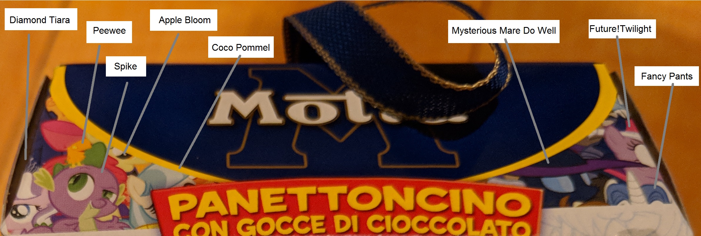
…and no Applejack.

Strike the “Chinese food in Rome” thing. This right here is a What the hell were you thinking? moment. Applejack certainly isn’t that popular, but come on, she’s part of the main ensemble! There are plenty of Applejack fans!

This is funny at a meta-level, because people like to joke Applejack is “the best background pony”, but it’s sad for fans that have to see her getting treated as a second-level citizen. Either this is a mistake of colossal proportions, or Applejack is just that unappealing of a character. I’ll be generous and go with the former.
I’ve bought other MLP merchandise, but it’s primarily been fan-created merchandise. Fan merchandise tends to match the quality I expect, because it’s made by people who actually care about getting the details right.
Look, Hasbro, just do it better next time, alright?