Similar to Wasserstein GAN, this is another theory-motivated paper with neat applications to deep learning. Once again, if you are looking for proof details, you are better off reading the original paper. The goal of this post is to give background and motivation.

Why Is This Paper Important?

Hyperparam optimization is a weird problem because everybody has to do it and nobody really likes it. The common options are either grid search, random search, or line search if your parameter is continuous. A mix of those does a pretty good job for most ML algorithms, even deep neural nets, which are a bit notorious for having many hyperparams.

However, I still think it’s worth keeping an eye on hyperparam optimization, for a couple reasons.

• If hyperparam optimization is better, more aspects of neural net design can be described as a hyperparam and automated. For example, the number of layers can be an explicit hyperparam, instead of something picked by hand. Right now, people don’t do this because it’s not worth doing for most problems, but the trend in research is that everybody pushes at the limits of their tools.
• Preliminary results like Neural Architecture Search suggests that there is learnable structure in neural net hyperparameters. It’s not yet applicable to anything, but I could see meta-learned models playing a bigger role in the future. At the same time, maybe we don’t need to throw a neural net at everything to get state-of-the-art results. (I like doing that as much as the next person, but machine learning doesn’t always have to mean deep learning.)
• There are simply a ton of interesting research questions that appear when each data point take hours or days to collect. Similar issues show up in robotics learning - robots are expensive and often need human supervision, which makes it hard to collect the ImageNet-scale datasets that neural nets are so good at.
• Better hyperparam optimization makes ML more accessible to others, because it reduces the amount of esoteric knowledge needed to get models to work. That’s good because people shouldn’t need to know that esoteric knowledge to solve their problems. It’s bad for me because weird deep learning expertise is one of the few things I’m good at, and I’m not sure I like knowing it could be obsolete down the line. All the more reason to pay attention.

Some Quick Background on Hyperparam Optimization

For two approachable introductions to the subject, I highly recommend two blog posts from Ben Recht’s blog, linked here and here. The key takeaways are

• Random search is a simple, deceptively strong baseline.
• Bayesian optimization can outperform random search by a bit.
• However, if you give random search twice the time, it beats a lot of Bayesian optimization methods. Yes, it’s more compute time, but sometimes buying more machines is easier than integrating clever ideas into your software stack.
• Successive halving (SH) is a nice extension of random search that lets you run many more hyperparams in the same amount of time, by pruning poor hyperparams early on. You have to be a little careful with how aggressively you prune, but in practice it does pretty well.
  • SH was later extended to the Hyperband algorithm, described here. Hyperband is one of the baseline methods used for comparison. Spearmint, a Bayesian optimization method, is the other main comparision.

Problem Setting

The paper focuses on discrete hyperparameter optimization. Generally, discrete optimization is trickier, and continuous problems can be approximated by discretizing the space, so I think this is an okay choice to make.

The paper further assumes all hyperparams are binary variables with value \(-1\) or \(+1\). Note you can still do things like allocate \(3\) hyperparams for the \(2^3 = 8\) different learning rates you want to try.

Let’s say there are \(n\) hyperparams. Then given all these assumptions, we want to learn a function \(f: \{-1,+1\}^n \to \mathbb{R}\), where the input is the hyperparam setting, and the output is the performance of the trained model. In the upcoming sections, we’ll use two different notations.

• \(f(x)\), in which case \(x = (x_1,x_2,x_3,\ldots, x_n)\) is some \(n\)-bit vector.
• \(f(x_1,x_2,\ldots,x_n)\), in which case we interpret \(f\) as a polynomial of \(n\) variables, where the variables equal either \(-1\) or \(+1\).

Polynomial Learning as Compressed Sensing

This is the key guiding framework of the algorithm. Viewing \(f(x)\) as a polynomial, we learn a sparse, low-degree polynomial \(g(x)\) that approximates \(f\).

What’s the intuition for why you’d want to do this? Well, to be honest, I have no idea why you’d decide to look at compressed sensing, instead of the other methods out there. But I can explain why it makes sense to me, after the fact.

To do better than random search, two things must be true.

• Your problem must have learnable structure.
• Your hyperparam optimization methods needs to discover and exploit that latent structure.

All of machine learning can be seen as fitting low-dimensional functions to inputs in high-dimensional space. This gets at why fitting a low-degree polynomial would make sense.

But then why include sparsity? Remember that we’re going to have very few data points, because each data point requires training a neural net to convergence. Sparsity helps with this by reducing the capacity of the polynomial fitting process - it stops it from putting a little bit of weight on thousands of different terms, which is one of the easiest ways to overfit. As a side effect, sparsity tends to make interpreting models easier.

(Aside: this is one of the common complaints about deep learning - it’s hard to interpret much out of the sum of 100 activations. But in practice, most deep learning problems have a lot of data, and enforcing sparsity just ends up hurting performance.)

When deriving the algorithm, we’ll assume that evaluating \(f(x)\) for a single \(x\) takes “a long time, but not too long”. By this, we mean functions run in \(\Omega(n^d)\) time for a somewhat large \(d\), but still run faster than things with exponential runtime.

The Parity Function Basis

To fit a low-degree polynomial, first note that the Boolean functions \(f: \{-1,+1\}^n \to \mathbb{R}\) form an inner product space. Define the inner product as

where the expectation is the uniform distribution over \(n\)-bit vectors. We can verify this satisfies the inner product definitions.

• Symmetry:

  \[\langle f, g\rangle = \mathbb{E}_{x} [f(x)g(x)] =\mathbb{E}_{x} [g(x)f(x)] = \langle g,f \rangle\]

• Linearity: for some constant \(a\),

  \[\langle af, g \rangle = \mathbb{E}_{x} [af(x)g(x)] = a \mathbb{E}_x [f(x)g(x) = a\langle f, g\rangle\]

  For functions \(f_1, f_2\),

  \[\langle f_1+f_2, g\rangle = \mathbb{E}_x[(f_1(x) + f_2(x))g(x)] = \mathbb{E}_x [f_1(x)g(x)] + \mathbb{E}_x [f_2(x)g(x)] = \langle f_1, g\rangle + \langle f_2, g\rangle\]

• Positive definiteness.

  \[\langle f, f\rangle = \mathbb{E}_x[f(x)^2] \ge 0\]

For \(\langle f, f\rangle\) to be \(0\), note \(f(x)^2 \ge 0\), so the only way for \(\mathbb{E}_x[f(x)]\) to equal \(0\) is if \(f(x) = 0\) everywhere.

Next, we want to find an orthonormal basis for this inner product space. For these functions, there’s a well known example. Let \(S \subset [n]\) be a subset of indicies \(1\) to \(n\). Define \(f_S(x)\) as

The functions \(\{f_S\}\) (known as the parity functions) form an orthonormal basis.

Why is this an orthonormal basis? A set \(\{f_1, f_2, \ldots, f_n\}\) is orthonormal if it satisfies two properties.

• For every \(f_i\), \(\langle f_i, f_i \rangle = 1\).
• For every \(f_i, f_j\) where \(i \neq j\), \(\langle f_i, f_j \rangle = 0\).

Now, we show the parity functions have this property.

In the upcoming sections, sometimes \(i\) means an index from \(1\) to \(n\), and sometimes \(i\) means a number from \(0\) to \(2^{n-1}\) that should be interpreted as \(n\) bits of binary. It should be inferable from context.

• By definition, \(\langle f_i, f_i \rangle = \mathbb{E}[f_i(x)^2]\). Note that \(f_i(x) = -1\) or \(f_i(x) = 1\), depending on how many matching bits there are between \(i\) and \(x\). In either case, \(f_i(x)^2 = 1\), so \(\langle f_i, f_i \rangle = 1\).
• For any two different subsets \(S_1, S_2\), there exists some \(i\) in one, but not the other. Without loss of generality, let \(i \in S_1\) and \(i \notin S_2\). We can write \(f_{S_1}(x)\) as

Take the expectation over \(x\), and factor it into the conditional expectation on \(x_i\).

The inner expectation equals \(c\), for some constant \(c\) that doesn’t depend on \(x_i\). Thus we can write the expectation as

Thus, the set is orthonormal. This leaves showing they form a basis. For this, note that there’s an isomorphism between functions \(f: \{-1, +1\}^n \to \mathbb{R}\) and vectors in \(\mathbb{R}^{2^n}\), where the mapping is

Isomorphisms preserve dimensionality, so the function space must have. must have dimension \(2^n\). There are \(2^n\) different subsets of \(\{1,\ldots,n\}\), so the parity functions must span the entire space. \(\blacksquare\)

Low Degree Approximation

Because the parity functions form an orthonormal basis, any function over \(\{-1, +1\}^n\) can be decomposed into a sum of parity functions, where the coefficient comes from the inner product. Let \(P(n)\) be the set of all subsets of \(1\) to \(n\). Then for any \(f\),

At this point we draw a comparison to Fourier series to build some intuition. Any periodic signal \(s(t)\) that’s sufficiently well behaved can be decomposed into a sum of sinusoids. The sinusoids \(\{1, \sin(t), \cos(t), \sin(2t), \cos(2t), \ldots \}\) form an orthonormal basis (which you can prove by throwing enough trigonometry identities at the problem.)

Intuitively, the earlier terms represent low-frequency components of the signal, and the later terms represent high-frequency components. To reconstruct \(s(t)\) exactly, we should do.

We can’t compute this exactly because the sum is infinite. However, we can approximate the signal by truncating the sum at some maximum \(N\)

This corresponds to dropping all the high frequency terms. Depending on the signal, this can still be a pretty good approximation.

Now, apply the same motivation to modeling \(f(x)\). We can write \(f\) as

Computing this exactly is intractable because there are \(2^n\) subsets. However, note that each term \(f_S(x_1,\ldots,x_n)\) is the product over a choice of indices. When \(S = \emptyset\), we get a \(0\)-degree constant term. When \(S\) is all numbers from \(1\) to \(n\), we get an \(n\)-degree term.

This reduces the number of terms from \(2^n\) to \(O(n^d)\), turning an exponentially big problem into a polynomially big one.

The approximation above is the best \(d\)-degree approximation, if you measure approximation error between \(f\) and \(g\) as \(\langle f-g, f-g\rangle = \mathbb{E}[(f-g)^2]\). But the best approximation isn’t necessarily a sparse one, and once we enforce sparsity, is a good approximation guaranteed to still exist? It turns out the answer is yes. From the paper:

Fact 4. [Man94] Let \(f\) be such that \(L_1(f) \le s\). Then there exists \(g\) such that \(g\) is \(s^2/\epsilon\) sparse and \(\mathbb{E}[(f-g)^2] \le \epsilon\). Function \(g\) is constructed by taking all coefficients of magnitude \(\epsilon/s\) or larger in \(f\)’s expansion as a polynomial.

Not only does this guarantee that a sparse approximation \(g\) exists, if \(f\) is a \(d\)-degree polynomial, \(g\) is also guaranteed to be degree \(d\), because it is formed by selecting terms that already exist in \(f\), and those terms must be degree \(d\) or lower.

Polynomial Recovery Algorithm

Let’s assume we have evaluations of \(f\) at \(T\) different points \(x_i\). The first trick for fitting a sparse polynomial is a classic: formulate the problem as a linear regression problem in a larger feature space. There are \(O(n^d)\) features, one for each subset \(S\) with \(|S| \le d\). We want to find coefficients \(\alpha_S\) that minimize the mean squared error.

To encourage sparsity, we apply another classic solution - add L1 regularization.

After solving this, we take the \(s\) coefficients with the largest magnitude, where \(s\) is a hyperparam for how sparse we want the polynomial to be.

(Yes, the hyperparam optimization method itself has hyperparams. It’s great.)

This gives the main subroutine, called Polynomial Sparse Recovery.

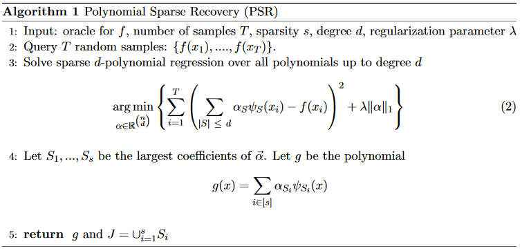
When called, it returns a sparse polynomial \(g\), and the set of all variables \(J\) that \(g\) depends on.

Runtime Bound For PSR

Let \(f\) be an \((\epsilon, d, s)\)-bounded function. Let \(\{H_S\}\) be an orthonormal polynomial basis bounded by \(K\). Then the PSR algorithm finds a \(g\) that’s within \(\epsilon\) of \(f\) in time \(O(n^d)\) with sample complexity \(T = \tilde{O}(K^2s^2 \log N/\epsilon)\).

In this statement, \(N\) is the size of the polynomial basis. For the special case of parity functions, we have \(K = 1\) and \(N = O(n^d)\), giving \(T = \tilde{O}(s^2 d \log n / \epsilon)\).

See paper for the proof.

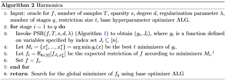
Harmonica: The Full Algorithm

We assume \(f\) is the error %, and that we want to minimize it. Sample some values \(f(x_i)\) by training some models, and fit a sparse polynomial \(g\).

Since \(g(x)\) has at most \(s\) terms, each of which is degree \(d\), it can depend on at most \(sd\) different variables. With the right choice of \(s,d\), brute forcing all \(2^{sd}\) possibilities is small enough to be doable. Note that \((2^s)^d\) is likely dwarfed by the \(O(n^dT)\) runtime for doing the linear regression.

However, this only gives settings for the variables \(J\) that \(g\) depends on. Thus, the full algorithm proceeds in stages. At each stage, we fit a sparse polynomial \(g\), find the settings that minimize \(g\), freeze those hyperparams, then iterate in the smaller hyperparam space. Applying this multiple times shrinks the hyperparam space, until it’s small enough to use a baseline hyperparam optimization method, like random search or successive halving.

(In practice, the authors find the \(t\) best settings instead of just the best one, then pick one of those \(t\) at random in the later stages. For example, if \(n=30\), \(t = 4\) and stage 1 decided values for 10 hyperparams, in stage 2 we sample one of the \(t\) settings to deciding the first 10, then sample randomly for the remaining 20.)

Experiments

The problem used is CIFAR-10, trained with a deep Resnet model. The model has 39 hyperparams, deciding everything from learning rate to L2 regularization to connectivity of the network, batch size, and non-linearity. To make the problem more difficult, 21 dummy hyperparams are added, giving 60 hyperparams total.

Harmonica is evaluated with 300 samples at each stage (meaning 300 trained models), with degree \(d = 3\), sparsity \(s=5\), and \(t=4\). They perform 2-3 stages of PSR (depending on the experiment), and use successive halving as the base hyperparam optimizer.

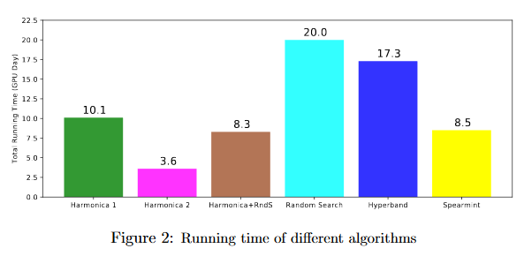
Results Summary

Harmonica outperforms random search, Hyperband and Spearmint.

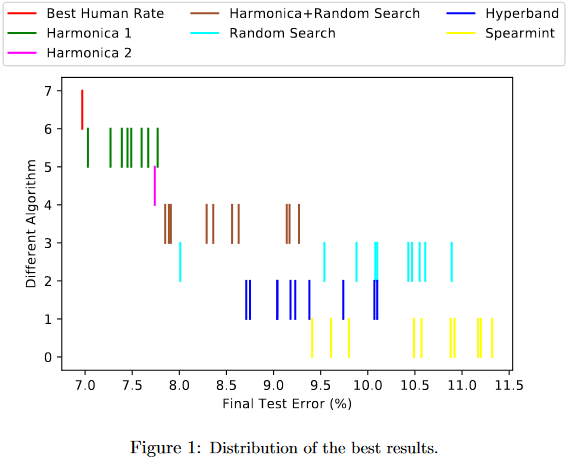
In this plot, the different between Harmonica 1 and Harmonica 2 is that in Harmonica 2, the final stage is given less time. This gives worse performance, but better runtime. The faster version (Harmonica 2) runs 5x faster than Random Search and outperforms it. The slower version (Harmonica 1) is still competitive with other approaches in runtime while giving much better results. Even when the base hyperparam optimizer is random search instead of successive halving, it outperforms random search in under half the time.

As Harmonica discovers settings for the important hyperparams, the average test error in the restricted hyperparam space drops. Each stage gives another drop in performance, but the drop is small between stage 2 and stage 3 - I’m guessing this is why they decided to only use 2 stages in the timing experiments.

To show that the chosen terms are meaningful, the coefficients in each stage are sorted by magnitude, to show which hyperparams influence error the most. Results are shown for a 3-stage Harmonica experiment, where sparsity \(s = 8\) for the first 2 stages and \(s = 5\) for the 3rd stage.

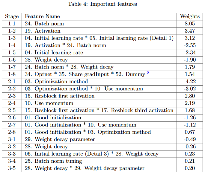
The minimizing settings often line up with human convention. Batch norm should be on (vs off), the activation function should be ReLU (vs sigmoid or tanh), and Adam should be used (vs SGD).

Many of the important hyperparams line up with convention - batch norm should be one, the activation function should be ReLU, and Adam is a better optimizer than SGD. Check the original paper for more details on the hyperparam definition.

One especially interesting term is the one discovered at stage 1-8. The dummy variable is extra and can be ignored. The authors say that in their code, if Optnet and Share gradInput are both true, training becomes unpredictable. The learned \(g\) is minimized if this term equals \(-1\), which happens if only one of Optnet and Share gradInput is true at a given time.

Advantages

In each stage of Harmonica, each model can be evaluated in parallel. By contrast, Bayesian optimization techniques are more difficult to parallelize because the derivation often assumes a single-threaded evaluation.

Enforcing hyperparam sparsity leads to interpretability - weights of different terms can be used to interpret which hyperparams are most important and least important. The approach successfully learned to ignore all dummy hyperparams.

Disadvantages

A coworker mentioned that Harmonica assumes a fixed computation budget for each stage, which doesn’t make it as good in an anytime setting (which is a better fit for Bayesian optimization.)

My intuition says that this approach works best when you have a large number of hyperparameters and want to initially narrow down the space. Each stage requires hundreds of models, and in smaller hyperparam spaces, evaluating 100 models with random search is going to enough tuning already. That being said, perhaps you can get away with fewer if you’re working in a smaller hyperparam space.

In the first two stages, Harmonica is run on a smaller 8 layer network, and the full 56 layer Resnet is only trained in the final stage. The argument is that hyperparams often have a consistent effect as the model gets deeper, so it’s okay to tune on a small network and copy the settings to a larger one. It’s not clear whether a similar trick was used in their baselines. If they weren’t, the runtime comparisons arne’t as impressive as they look.

The approach only works if it makes sense for the features to be sparse. This isn’t that big a disadvantage, in my experience neural net hyperparams are nearly independent. This is backed up by the Harmonica results - the important terms are almost all degree 1. (The authors observed that they did need \(d \ge 2\) for best performance.)

The derivation only works with discrete, binary features. Extending the approach to arbitrary discrete hyperparams doesn’t look too bad (just take the closest power of 2), but extending to continuous spaces looks quite a bit trickier.

Closing Thoughts

Overall I like this paper quite a bit. I’m not sure how practical it is - the “tune on small, copy to large” trick in particular feels a bit sketchy. But that should only affect the runtime of the algorithm, not the performance. I think it’s neat that it continues to work in empirical land.

One thing that’s nice is that because the final stage can use any hyperparam optimization algorithm, it’s easy to mix-and-match Harmonica with other approaches. So even if Harmonica doesn’t pan out in further testing, the polynomial sparse recovery subroutine could be an interesting building block in future work.