The Other Two Envelope Problem
The two envelope problem is a famous problem from decision theory, at least famous enough to have its own Wikipedia page. It’s an interesting problem, but this post is about its less well known variation.
Here is the formulation.
There are two envelopes, one with \(A\) and one with \(B\) dollars, \(A \neq B\). \(A\) and \(B\) are unknown positive integers. You are randomly given an envelope, can look inside, then must choose whether to switch envelopes or not.
Does there exists a switching strategy which ends with the larger envelope more than half the time?
At first glance, the answer should be no. Although we know the contents of one envelope, we have no information on how much the other envelope might have. When the other envelope is a black box, how can we make a meaningful decision?
As it turns out, such a strategy does exist, and the small amount of information we have (the amount in the current envelope) is enough to improve our standing, even when the alternative has unknown value.
The Power of Randomness
The trick is to make the switching decision randomly, in a way that biases outcomes to end with the larger envelope. The strategy is as follows:
- Inspect amount \(X\) inside the envelope.
- Flip a fair coin until it lands tails.
- If there were at least \(X\) flips, switch envelopes. Otherwise, do not switch.
For analysis, assume without loss of generality that \(A < B\). There are two ways to end with envelope \(B\). Either start with \(A\) and switch, or start with \(B\) and do not switch. The first case happens with probability
\[P[\text{started A, switched}] = \frac{1}{2}\left(\frac{1}{2^{A}}\right)\]The second happens with probability
\[P[\text{started B, did not switch}] = \frac{1}{2}\left(1 - \frac{1}{2^{B}}\right)\]So, the chance to end with \(B\) is
\[\frac{1}{2} + \frac{1}{2^{A+1}} - \frac{1}{2^{B+1}}\]which is indeed larger than \(1/2\) for \(A < B\). \(\blacksquare\)
Extending to the Reals
This coin flip strategy works when \(A\) and \(B\) are integers, but fails when \(A,B\) are arbitrary reals. The problem is that the number of flips comes from a discrete distribution, so it does not have the granularity to distinguish between values like \(A = 2.3, B = 2.4\).
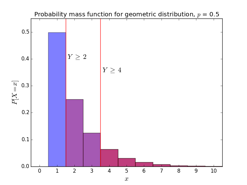
So, how is this strategy extendable? The way the current strategy works is by creating a decision boundary based on the amount in the seen envelope. The boundary is then applied to the geometric distribution with parameter \(p=1/2\).

Decision boundaries when \(A = 2, B = 4\). The switching strategy gets an advantage when the sampled \(Y\) lies between the two boundaries.
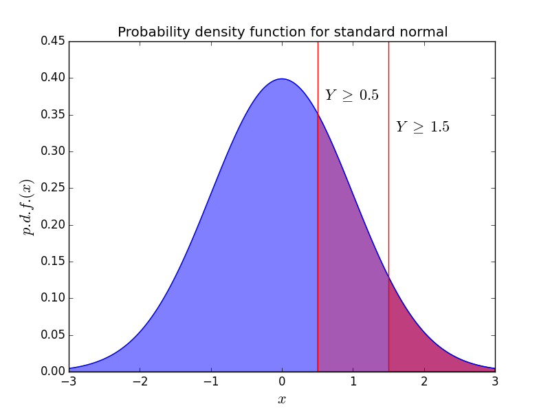
To handle arbitrary reals, we should use a continuous probability distribution instead. Nothing in the previous logic relies on the distribution being discrete, so we can simply drop in a distribution of our choice. The only requirement we need is a strictly positive probability density function over \((-\infty, \infty)\) (we’ll explain why we need this later.) The standard normal distribution \(N(0, 1)\) will do fine.
The modified strategy is
- Inspect amount \(X\) inside the envelope.
- Sample \(Y\) from \(N(0,1)\).
- If \(Y \ge X\). switch. Otherwise, do not switch.

Decision boundaries when \(A=0.5, B=1.5\). Again, the switching strategy gets an advantage when \(Y\) falls between \(A\) and \(B\).
The proof is also similar. For \(A < B\), \(P(Y \ge A) > P(Y \ge B)\). This is why the p.d.f. needs to be positive everywhere. If the p.d.f. is zero over some interval \([a,b]\), it is possible that both \(A, B \in [a,b]\), which gives \(P(Y \ge A) = P(Y \ge B)\). The chance of ending with the larger envelope is
\[\frac{1}{2}P(Y \ge A) + \frac{1}{2}\left(1 - P(Y \ge B)\right) = \frac{1}{2} + \frac{1}{2}\left(P(Y \ge A) - P(Y \ge B)\right) > \frac{1}{2}\]and this strategy generalizes to real valued envelopes. \(\blacksquare\)
Extending to Multiple Envelopes
At this point, it’s worth considering whether we can take any lessons from this problem. If we substitute “given an envelope” with “given an action”, and “dollars” with “utility”, this result suggests that even with no information on alternative choices, we could use a random action to improve our current standing. In real life, we often have very little information on how different actions will play out, so this power to bias towards improvement is appealing. However, in real life there are usually much more than two possible actions, so we should first consider whether the two envelope framework is even valid.
When there are \(n\) envelopes instead of \(2\) envelopes, we can no longer aim for only the best envelope. The switch could slightly help us, slightly hurt us, especially help us, or especially hurt us. Because of this, we need to modify the criteria of a good strategy.
There are \(n\) envelopes, which give utilities \(A_1 < A_2 < A_3 < \cdots < A_n\). The \(A_i\) are unknown real numbers. You are randomly given an envelope, can look inside, then must choose whether to switch with another envelope.
Does there exist a switching strategy that improves your utility more often than it worsens your utility?
Once again, it turns out the real valued two envelope strategy still works with appropriate modifications. We still choose whether to swap by seeing if sample \(Y\) is greater than seen utility \(X\). The only difference is choosing which envelope to switch to. From the opener’s perspective, every other envelope appears identical. Thus, if the strategy says to swap, we should pick an alternative envelope at random.
This leaves showing the improvement chance is higher than the worsening chance. If the algorithm does not swap, the utility is unchanged, so it suffices to analyze only situations where we switch envelopes.
For envelope \(i\), the chance of switching is \(P[Y \ge A_i]\). The reward rises for \(n-i\) envelopes and drops for \(i-1\) envelopes. Thus, the chance of improving utility is
\[P[\text{utility rises}] = \sum_{i=1}^n \frac{1}{n} P[Y \ge A_i]\cdot \frac{n-i}{n-1}\]and the chance of worsening utility is
\[P[\text{utility drops}] = \sum_{i=1}^n \frac{1}{n} P[Y \ge A_i]\cdot \frac{i-1}{n-1}\]Envelope \(i\) has \(n-i\) envelopes that are better, and envelope \(n-i+1\) has \(n-i\) envelopes that are worse. Intuitively, every improving term for \(A_i\) should cancel with a worsening term for \(A_{n-i+1}\), but the improving terms have more weight because the switching probability after observing \(A_i\) is higher. This is formalized below.
Take the difference and pair up terms with matching \(P[Y \ge A_i]\) to get
\[P[\text{improves}] - P[\text{worsens}] = \frac{1}{n}\sum_{i=1}^n \frac{n-2i+1}{n-1} P[Y \ge A_i]\]The coefficients of the terms are \(\frac{n-1}{n-1}, \frac{n-3}{n-1}, \ldots, \frac{-(n-3)}{n-1}, \frac{-(n-1)}{n-1}\). Since we only care about whether the difference is positive, multiply by \(2\) to get two copies of the terms, then pair terms by coefficient, matching each coefficient with its negative.
\[2(P[\text{improves}] - P[\text{worsens}]) = \frac{1}{n}\sum_{i=1}^n \frac{n-2i+1}{n-1} (P[Y \ge A_i] - P[Y \ge A_{n+1-i}])\]Consider each term of this summation.
- For \(i < \frac{n+1}{2}\), the coefficient is positive, and \(A_i < A_{n+1-i}\), so \(P[Y \ge A_i] - P[Y \ge A_{n+1-i}]\) is positive. The entire term is positive.
- For \(i = \frac{n+1}{2}\), the coefficent is \(0\).
- For \(i > \frac{n+1}{2}\), the coefficient is negative, and \(A_i > A_{n+1-i}\), so \(P[Y \ge A_i] - P[Y \ge A_{n+1-i}]\) is negative. The entire term is positive.
Every term in the summation is positive or zero, so the entire sum is positive, and the probability of increasing utility is higher than the probability of decreasing it. \(\blacksquare\)
Implications
So, now we have a strategy that is very slightly biased towards increasing utility. But before trying to implement this in real life, it’s worth thinking through all the complications.
- The values \(A_i\) are chosen through some unknown process. Although this strategy is more likely to end on a larger \(A_j\), it is impossible to quantify how much better your utility will be after the swap. The utility might even go down in expectation. Although the chance of improving utility is higher, the potential utility increase may be small while the potential utility decrease is large. If we had more information about how \(A_j\) are generated, then we could argue this in more detail, but at that point this information independent scheme is probably no longer useful.
- The analysis relies on having a value on the initial action. It is incredibly likely that we are just as confused about the value of our current action as we are about the values of other actions, which renders the strategy moot.
- The analysis also relies on starting with an action picked uniformly at random out of a pool of possible actions. In reality, this is almost never the case. We usually have reasons to choose to act in one way or another, which places a non-uniform prior on the initial action. Intuitively, if we are already good at making decisions, it is far less likely we can switch to an even better one.
So overall, this is not a life hack. All we have is a surprising decision theory result, and that’s fine too.
(Thanks to the people who helped review earlier drafts.)