Appendix: A Batch Norm Overview
What Is Batch Norm?
Batch norm is motivated by “internal covariate shift”. What does that mean? Well, let’s suppose we’re training a neural network on some data. The input will go through a few hidden layers, then go to the output.
Adapted from a picture from CS231N
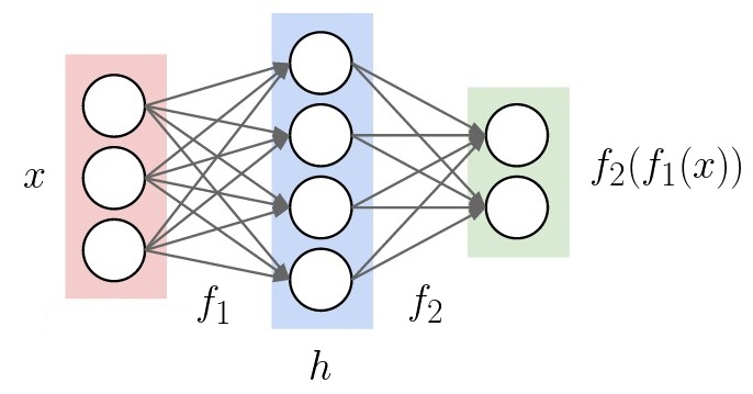
At train time, each layer has a different job. The 1st layer’s job is to learn good features from the input. The 2nd layer’s job is to learn good features from the 1st layer’s features. We only have the two layers here, but if there was a 3rd, the 3rd layer’s job would be learning features from the 2nd layer. This continues up to the output layer, whose job is to solve the task from the last layer’s features.
(If you prefer function notation, \(f_1\) learns from \(x\), and \(f_2\) learns from \(h = f_1(x)\).)
Each of these jobs depends on the other ones, so we can’t optimize each independently. Luckily, backprop gives a way to compute the parameter update for all layers at once. Easy, right?
As the parameters change, the distribution of each layer’s activations changes too. This makes the next layer’s job harder, because the distribution it’s learning from keeps changing underneath it. Each layer must continually adapt to the distribution of the layer before it, and it seems like this should slow down learning. The literature calls this covariate shift. Generally, it’s been studied at the data level, where the test set distribution differs from the training set distribution.
The observation motivating batch norm is that even when the data is fine, we can still have internal covariate shift, thanks to layer activations shifting over time.
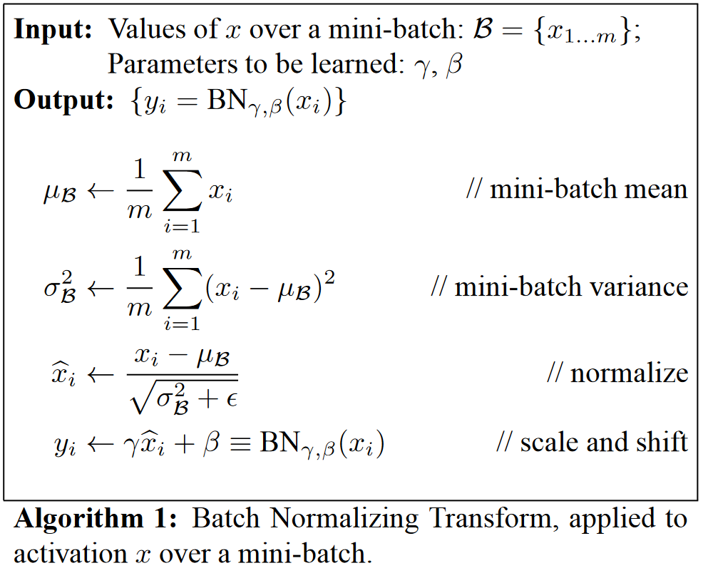
To address this, batch norm normalizes every output unit to be mean \(0\), variance \(1\). Well, kind of. There are some key details. (In the following, \(BN(x)\) is the batch norm function.)
To center the distribution of output \(x\), we compute the mean \(\mu\), the variance \(\sigma^2\), and transform \(x\) to
\[BN(x) = \frac{x - \mu}{\sqrt{\sigma^2}}\]Mean \(\mu\) and variance \(\sigma^2\) depend on the entire distribution, which is impractical to compute. So instead, we compute the mean and variance for just the minibatch \(\mathcal{B} = \{x_1, x_2,\ldots, x_m\}\).
\[\mu_\mathcal{B} = \sum_{i=1}^m x_i\] \[\sigma^2_\mathcal{B} = \sum_{i=1}^m (x_i - \mu_B)^2\] \[BN(x_i) = \frac{x_i - \mu_B}{\sqrt{\sigma_\mathcal{B}^2 + \epsilon}}\](The \(\epsilon\) is here to avoid division by zero problems.)
Note \(BN(x_i)\) now depends on other \(x_j\) in the minibatch!
Finally, in practice we don’t want to limit the output distribution to always be mean 0 and variance 1, because this constrains the network too much for learning. We define
\[y = \gamma BN(x) + \beta\]to be the actual output, and let \(\beta\) and \(\gamma\) be learnable parameters.
To make the output deterministic at eval time, we keep an exponential moving average of \(\mu_\mathcal{B}\) and \(\sigma^2_\mathcal{B}\). At every step, we also compute
\[\mu \gets (1-\alpha) \mu + \alpha \mu_\mathcal{B}\] \[\sigma^2 \gets (1-\alpha) \sigma^2 + \alpha\sigma^2_\mathcal{B}\]The exponential moving average has a few nice properties: it places more weight on recent inputs, it doesn’t require much additional memory, and because the update is a simple addition, it doesn’t take much time either.
When the network converges, the moving average is usually a good estimate of the dataset-wide mean and variance. At test time, We normalize with the averaged \(\mu\) and \(\sigma\) instead. This makes each \(x_i\) independent again.
\[BN_{test}(x) = \frac{x - \mu}{\sqrt{\sigma^2 + \epsilon}}\]Note that thanks to \(\gamma\) and \(\beta\), the activations can follow any distribution. (When \(\gamma = \sqrt{\sigma_{\mathcal{B}}^2 + \epsilon}\) and \(\beta = \mu_{\mathcal{B}}\), batch norm is the identity function.) This kind of breaks the internal covariate shift argument. If the network can still learn any distribution, how have we helped fix the problem?
My theory is that the answer lies in how the distribution is represented. Consider just the shaded unit below.
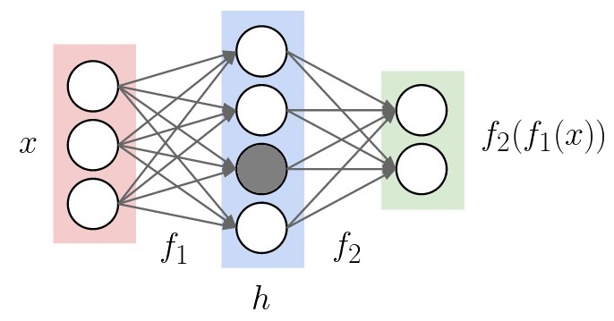
After applying batch norm, this unit has mean \(\beta\), variance \(\gamma\). The statistics of the distribution are concentrated entirely into those two variables. If batch norm wasn’t used, the mean and variance would be implicitly defined by the weights along the arrows flowing into the shaded unit. When mean and variance are directly optimizable, it’s easier for gradient descent to discover the best distribution for each layer’s activations.
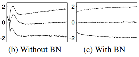
A plot of the 15th, 50th, and 85th percentiles of an activation’s distribution when trained on MNIST. Note that the batch norm plot is more stable. Also note that both distributions converge to a similar point, but batch norm gets close to the final distribution much sooner.