Simulating a Biased Coin With a Fair One
Suppose you need to simulate an event that happens \(p = 1/4\) of the time, and all you have is a fair coin. Well, that’s easy enough. Flip the coin twice. Report success if you get 2 heads, and report failure otherwise.
Suppose \(p = 1/3\) instead. That may not be a power of 2, but there is still a simple solution. Flip the fair coin twice. Report success on HH, report failure on HT or TH, and try again on TT. Each iteration takes \(2\) coin flips, and there is a \(3/4\) probability of halting, giving \(8/3\) expected coin flips.
Now, suppose you need to simulate \(p = 1/10^{100}\). Well, nothing is especially wrong with the current scheme. We need \(\lceil\log_2(10^{100})\rceil = 333\) coin flips to get enough outcomes. Then, label \(1\) case as success, \(10^{100} - 1\) as failure, and the rest as retries. For analyzing runtime, these numbers are starting to get messy, but we can at least ballpark the expected number of flips. The probability of halting is \(> 1/2\), since by construction \(2^{332} < 10^{100} < 2^{333}\), meaning the number of retry cases is less than half of all cases. Thus, the expected number of flips is at most \(666\). Yes, that is…
(•_•) ( •_•)>⌐■-■ (⌐■_■)
a devilish upper bound, but things could be worse.
(I’m not sorry.)
But, what if you need to simulate \(p = 1 / 10^{10^{100}}\)? Or simulate \(p = 1/\pi\)? In the first case, the number of flips needed is enormous. In the second, the scheme fails completely - there is no way to simulate irrational probabilities.
Easy Optimizations
We’ll get back to the irrational case later.
Recall how we simulated \(p=1/4\). The scheme reports success only on HH. So, if the first flip lands tails, we can halt immediately, since whatever way the second coin lands, we will report failure anyways. The revised algorithm is
- Flip a coin. If tails, report failure.
- Flip a coin. Report success on heads and failure on tails.
This gives \(3/2\) expected flips instead of \(2\) flips.
As another example, consider \(p = 1/5\). First, plan to flip 3 coins. Divide the 8 outcomes into 1 success case, 4 failure cases, and 3 retry cases. These can be distributed as
- accept: HHH
- failing: THH, THT, TTH, TTT
- retry: HHT, HTH, HTT
If the first coin is T, we can stop immediately. If the first two coins are HT, we can retry immediately. The only case left is HH, for which we need to see the third flip before deciding what to do.
(Some of you may be getting flashbacks to prefix-free codes. If you haven’t seen those, don’t worry, they won’t show up in this post.)
With clever rearrangement, we can bundle outcomes of a given type under as few unique prefixes as possible. This gives some improvement for rational \(p\), but still does not let us simulate irrational \(p\). For this, we need to switch to a new framework.
A New Paradigm
I did not come up with this method - I discovered it from here. I wish I had come up with it, for reasons that will become clear.
Let \(p = 0.b_1b_2b_3b_4b_5\ldots\) be the binary expansion of \(p\). Proceed as follows.
- Flip a coin until it lands on heads.
- Let \(n\) be the number of coins flipped. Report success if \(b_n = 1\) and report failure otherwise
The probability the process stops after \(n\) flips is \(1/2^n\), so the probability of success is
\[P[success] = \sum_{n: b_n = 1}^\infty \frac{1}{2^n} = p\]Regardless of \(p\), it takes \(2\) expected flips for the coin to land heads. Thus, any biased coin can be simulated in \(2\) expected flips. This beats out the other scheme, works for all \(p\) instead of only rational \(p\), and best of all you can compute bits \(b_i\) lazily, making this implementable in real life and not just in theory.
Slick, right? This idea may have been obvious to you, but it certainly wasn’t to me. After thinking about the problem more, I eventually recreated a potential chain of reasoning to reach the same result.
Bits and Pieces
(Starting now, I will use \(1\) interchangeably with heads and \(0\) interchangeably with tails.)
Consider the following algorithm.
- Construct a real number in \([0,1]\) by flipping an infinite number of coins, generating a random number \(0.b_1b_2b_3\ldots\), where \(b_i\) is the outcome of coin flip \(i\). Let this number be \(x\).
- Report success if \(x \le p\) and failure otherwise.
This algorithm is correct as long as the decimals generated follow a uniform distribution over \([0, 1]\). I won’t prove this, but for an appeal to intuition: any two bit strings of length \(k\) are generated with the same probability \(1/2^k\), and the numbers these represent are evenly distributed over the interval \([0, 1]\). As \(k \to\infty\) this approaches a uniform distribution.
Assuming this all sounds reasonable, the algorithm works! Only, there is the small problem of flipping \(\infty\)-ly many coins. However, similarly to the \(p = 1/4\) case, we can stop coin flipping as soon as as it is guaranteed the number will fall in or out of \([0, p]\).
When does this occur? For now, limit to the case where \(p\) has an infinite binary expansion. For the sake of an example, suppose \(p = 0.1010101\ldots\). There are 2 cases for the first flip.
-
The coin lands \(1\). Starting from \(0.1\), it is possible to fall inside or outside \([0,p]\), depending on how the next flips go. The algorithm must continue.
-
The coin lands \(0\). Starting from \(0.0\), it is impossible to fall outside \([0,p]\). Even if every coin lands \(1\), \(0.0111\ldots_2 = 0.1_2 < p\). (This is why \(p\) having an infinite binary expansion is important - it ensures there will be another \(1\) down the line.) The algorithm can halt and report success.
So, the algorithm halts unless the coin flip matches the \(1\) in \(p\)’s expansion. If it does not match, it succeeds. Consider what happens next. Starting from \(0.1\), there are 2 cases.
- Next coin lands \(1\). Since \(0.11 > p\), we can immediately report failure.
- Next coin lands \(0\). Similarly to before, the number may or may not end in \([0,p]\), so the algorithm must continue.
So, the algorithm halts unless the coin flip matches the \(0\) in \(p\)’s expansion. If it does not match, it fails. This gives the following algorithm.
- Flip a coin until the \(n\)th coin fails to match \(b_n\)
- Report success if \(b_n = 1\) and failure otherwise.
Note this is essentially the same algorithm as mentioned above! The only difference is the ending condition. Instead of halting on heads, the algorithm halts if the random bit does not match the “true” bit. Both happen \(1/2\) the time, so the two algorithms are equivalent.
(If you wish, you can extend this reasoning to \(p\) with finite binary expansions. Just make the expansion infinite by expanding the trailing \(1\) into \(0.1_2 = 0.0111\ldots_2\).)
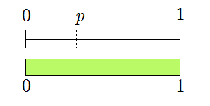
Here’s a sample run of the algorithm told in pictures. The green region represents the possible values of \(x\) as bits are generated. Initially, any \(x\) is possible.
The first generated bit is \(0\), reducing the valid region to
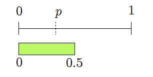
This still overlaps \([0,p]\), so continue. The second bit is \(1\), giving
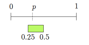
This still overlaps, so continue. The third bit is \(1\), giving
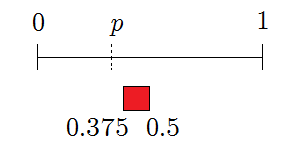
The feasible region for \(x\) no longer intersects \([0,p]\), so the algorithm reports failure.
CS-minded people may see similarities to binary search. Each bit chooses which half of the feasible region we move to, and the halving continues until the feasible region is a subset of \([0,p]\) or disjoint from \([0,p]\).
Proving Optimality
This scheme is very, very efficient. But, is it the best we can do? Is there an algorithm that does better than \(2\) expected flips for general \(p\)?
It turns out that no, \(2\) expected flips is optimal. More surprisingly, the proof is not too bad.
For a given \(p\), any algorithm can be represented by a computation tree. That tree encodes whether the algorithm succeeds, fails, or continues, based on the next bit and all previously generated bits.
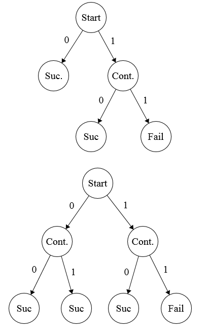
Two sample computation trees for \(p = 3/4\).
With the convention that the root is level \(0\), children of the root are level \(1\), and so on, let the weight of a node be \(1/2^{\text{level}}\). Equivalently, the weight is the probability the algorithm reaches that node.
For a given algorithm and \(p\), the expected number of flips is the expected number of edges traversed in the algorithm’s computation tree. On a given run, the number of edges traversed is the number of vertices visited, ignoring the root. By linearity of expectation,
\[E[flips] = \sum_{v \in T, v \neq root} \text{weight}(v)\]To be correct, an algorithm must end at a success node with probability \(p\). Thus, the sum of weights for success nodes must be \(p\). For \(p\) with infinitely long binary expansions, we must have an infinitely deep computation tree. If the tree had finite depth \(d\), any leaf node weight would be a multiple of \(2^{-d}\), and the sum of success node weights would have at most \(d\) decimal places.
Thus, the computation tree must be infinitely deep. To be infinitely deep, every level of the tree (except the root) must have at least 2 nodes. Thus, a lower bound on the expected number of flips is
\[E[flips] \ge \sum_{k=1}^\infty 2 \cdot \frac{1}{2^k} = 2\]and as we have shown earlier, this lower bound is achievable. \(\blacksquare\)
(For \(p\) with finite binary expansions, you can do better than \(2\) expected flips. Proving the optimal bound for that is left as an exercise.)
In Conclusion…
Every coin in your wallet is now an arbitrarily biased bit generating machine that runs at proven-optimal efficiency. If you run into a bridge troll who demands you simulate several flips of a coin that lands heads \(1/\pi\) of the time, you’ll be ready. If you don’t, at least you know one more interesting thing.